Clustering case¶

Run in Google Colab

%matplotlib inline

import pandas as pd
import matplotlib.pyplot as plt
import seaborn as sns 

from sklearn.preprocessing import StandardScaler
from sklearn.cluster import KMeans
from sklearn.cluster import AgglomerativeClustering

Case description¶

Suppose a financial technology (fintech) startup conducted an online survey and obtained data from 1010 individuals. All respondents agreed to receive marketing material from the company.

The data file responses.csv contains the data from the questionnaire and consists of 1010 rows (people) and 150 columns (139 integer and 11 categorical). See the data description PDF for a detailed overview of the data.

Let’s imagine that after the fintech startup collected the data, they realized that they forgot to include a question regarding wether the respondent is male or female. Since this information is vital to an upcoming marketing campaign which is targeted specifially at women, they decide to use two different clustering methods to figure out wether an individual is male or female based on their reported height and weight.

A) Data preparation

Import the data (responses.csv), call the DataFrame df and delete all observations with missing infomation (” df.dropna(inplace=True)”). - Next, create a new DataFrame called df_1 where you only select the variables Height, Weight and also Gender.
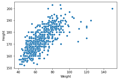
Visualize the variables Height and Weight in a scatterplot.

Note that we pretend the variable Gender is missing but select it anyway in order to compare the results from the clustering methods with the real gender our observations. However, it is important to note that in real use cases, the cluster analysis is performed if there are no Y-labels (like Gender) available.

B) Standardization

Create a new DataFrame (call it X) with only Height and Weight
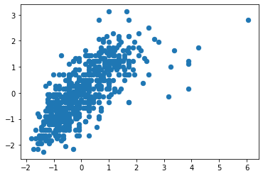
Standardize the variables (withStandardScaler), store them in a new DataFrame (called X_std)
Visualize the result in a scatterplot.

C) k-Means

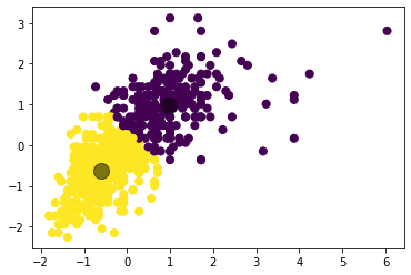
Use k-Means to determine the two clusters in the dataset X_std and visualize the result (label the two clusters as points with different colors and display the cluster centers).
Furthermore, save the result as a new variable (gender_kmeans) in the original DataFrame df.

D) Hierarchical Clustering (Ward)

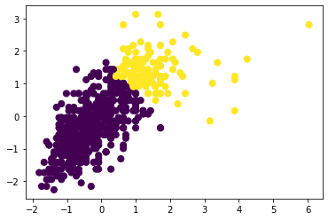
Apply hierarchical clustering with Ward’s method to the data (X_std)
Visualize the result (label the two clusters as points with different colors).
Furthermore, save the result as a new variable (gender_ward) in the original DataFrame df.

E) Scatterplots

Next, we use Seaborn to create three different separate scatterplots in which we visualize the variables Height and Weight together with

(1) the variable Gender (as points with different colors) from the DataFrame df,
(2) the variable gender_kmeans (as points with different colors) from the DataFrame df,
(3) the variable gender_ward (as points with different colors) from the DataFrame df.

See Seaborn’s documention to understand the syntax.

F) Comparision

a) What differences do you observe in the results? How do the clustering-results differ?

Now compare the result with the actual gender variable to the clusters of k-Means and hierarchical cluster analysis (note that this is not possible in real world cases since we usually don’t have true labels). Answer the following questions:

Which cluster method performed better if the company has the following goal:
b) address as many women as possible.

G) Data finalization

Assume the company decides to use the k-means clustering results. Hence, we create a new DataFrame called df_3 where we only keep observations which are labeled as female in the gender_kmeans result.

Solution¶

A) Data preparation¶

df = pd.read_csv("https://raw.githubusercontent.com/kirenz/datasets/master/responses.csv")
df.dropna(inplace=True)

df_1 = df[['Weight','Height','Gender']] 
df_1.info()

<class 'pandas.core.frame.DataFrame'>
Int64Index: 674 entries, 0 to 1009
Data columns (total 3 columns):
 #   Column  Non-Null Count  Dtype  
---  ------  --------------  -----  
 0   Weight  674 non-null    float64
 1   Height  674 non-null    float64
 2   Gender  674 non-null    object 
dtypes: float64(2), object(1)
memory usage: 21.1+ KB

sns.scatterplot(x='Weight', y='Height', data=df_1);

B) Standardization¶

# Standardization of features
X = df[['Weight','Height']] 

scaler = StandardScaler()
X_std = scaler.fit_transform(X)

plt.scatter(X_std[:, 0], X_std[:, 1], s=40);

C) k-Means¶

kmeans = KMeans(n_clusters=2)
kmeans.fit(X_std)

KMeans(n_clusters=2)

y_kmeans = kmeans.predict(X_std)

plt.scatter(X_std[:, 0], X_std[:, 1], c=y_kmeans, s=50, cmap='viridis')
centers = kmeans.cluster_centers_
plt.scatter(centers[:, 0], centers[:, 1], c='black', s=200, alpha=0.5);

df['gender_kmeans'] = y_kmeans

D) Hierarchical Clustering (Ward)¶

ward = AgglomerativeClustering(linkage='ward', affinity='euclidean', n_clusters=2)
ward.fit(X_std)

AgglomerativeClustering()

plt.scatter(X_std[:, 0], X_std[:, 1], c=ward.labels_, s=50, cmap='viridis');

gender_ward = ward.fit_predict(X_std)

df['gender_ward'] = gender_ward 

E), F) Compare results¶

sns.scatterplot(x='Weight', y='Height', hue='Gender', data=df);

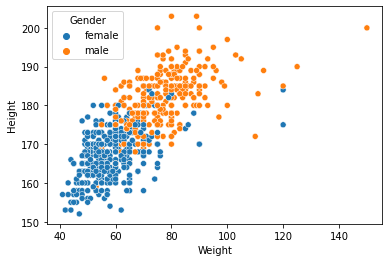
df['Gender'].value_counts()

female    402
male      272
Name: Gender, dtype: int64

# K means
sns.scatterplot(x='Weight', y='Height', hue='gender_kmeans', data=df);

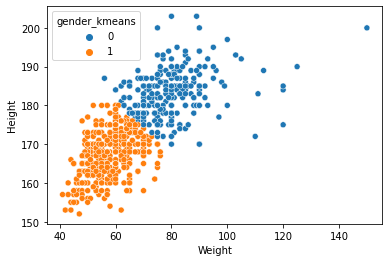
df['gender_kmeans'].value_counts()

1    413
0    261
Name: gender_kmeans, dtype: int64

#Ward
sns.scatterplot(x='Weight', y='Height', hue='gender_ward', data=df);

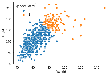
df['gender_ward'].value_counts()

0    548
1    126
Name: gender_ward, dtype: int64

G) Finalize data¶

df_3 = df[df.gender_kmeans == 1]
df_3.head()

	Music	Slow songs or fast songs	Dance	Folk	Country	Classical music	Musical	Pop	Rock	Metal or Hardrock	...	Weight	Number of siblings	Gender	Left - right handed	Education	Only child	Village - town	House - block of flats	gender_kmeans
0	5.0	3.0	2.0	1.0	2.0	2.0	1.0	5.0	5.0	1.0	...	48.0	1.0	female	right handed	college/bachelor degree	no	village	block of flats	1
1	4.0	4.0	2.0	1.0	1.0	1.0	2.0	3.0	5.0	4.0	...	58.0	2.0	female	right handed	college/bachelor degree	no	city	block of flats	1
2	5.0	5.0	2.0	2.0	3.0	4.0	5.0	3.0	5.0	3.0	...	67.0	2.0	female	right handed	secondary school	no	city	block of flats	1
4	5.0	3.0	4.0	3.0	2.0	4.0	3.0	5.0	3.0	1.0	...	59.0	1.0	female	right handed	secondary school	no	village	house/bungalow	1
6	5.0	5.0	5.0	3.0	1.0	2.0	2.0	5.0	3.0	1.0	...	50.0	1.0	female	right handed	secondary school	no	village	house/bungalow	1

5 rows × 152 columns

Clustering

Clustering case

Contents