First steps in pandas

This very short introduction to pandas is mainly based on the excellent pandas documentation.

To use this tutorial, I recommend the following procedure:

1. On your machine, create a new folder called pandas

2. Download this tutorial as .ipynb (on the top right of this webpage, select the download button) and move it to your pandas folder

3. Open Visual Studio Code and select the “Explorer” symbol on the top left in the Activity Bar

4. Select “Open Folder” and choose your folder pandas. This folder is now your project directory

5. In the Explorer, open the file pandas-intro-short.ipynb

Import pandas

• To load the pandas package and start working with it, import the package.

• The community agreed alias for pandas is pd, so loading pandas as pd is assumed standard practice for all of the pandas documentation:

import pandas as pd

Data creation

• To manually store data in a table, create a DataFrame:

# create the DataFrame and name it my_df

my_df = pd.DataFrame(
    { 
        'name': [ "Tom", "Lisa", "Peter"],
        'height': [1.68, 1.93, 1.72],
        'weight': [48.4, 89.8, 84.2],
        'gender': ['male', 'female', 'male'] 
        }
)

# show my_df
my_df

	name	height	weight	gender
0	Tom	1.68	48.4	male
1	Lisa	1.93	89.8	female
2	Peter	1.72	84.2	male

Import data

• pandas supports many different file formats or data sources out of the box (csv, excel, sql, json, parquet, …)

• each of them import data with the prefix read_*

• Import data, available as a CSV file in a GitHub repo:

df = pd.read_csv("https://raw.githubusercontent.com/kirenz/datasets/master/height_unclean.csv", delimiter=";", decimal=",")

# show head
df.head()

	Name	ID%	Height	Average Height Parents	Gender
0	Stefanie	1	162	161.5	female
1	Peter	2	163	163.5	male
2	Stefanie	3	163	163.2	female
3	Manuela	4	164	165.1	female
4	Simon	5	164	163.2	male

# same import with different style

ROOT = "https://raw.githubusercontent.com/kirenz/datasets/master/"
DATA = "height_unclean.csv"

df = pd.read_csv(ROOT + DATA, delimiter=";", decimal=",")

# show head
df.head()

	Name	ID%	Height	Average Height Parents	Gender
0	Stefanie	1	162	161.5	female
1	Peter	2	163	163.5	male
2	Stefanie	3	163	163.2	female
3	Manuela	4	164	165.1	female
4	Simon	5	164	163.2	male

Store data

• pandas supports many different file formats (csv, excel, sql, json, parquet, …)

• each of them stores data with the prefix to_*

• The following code will save data as an Excel file in your current directory (you may need to install OpenPyXL first.

Note

Anaconda installation of OpenPyXL):

• In the example here, the sheet_name is named people_height instead of the default Sheet1. By setting index=False the row index labels are not saved in the spreadsheet:

df.to_excel("height.xlsx", sheet_name="people_height", index=False)

• The equivalent read function read_excel() would reload the data to a DataFrame:

# load excel file
df_new = pd.read_excel("height.xlsx", sheet_name="people_height")

Viewing data

Overview

# show df
df

	Name	ID%	Height	Average Height Parents	Gender
0	Stefanie	1	162	161.5	female
1	Peter	2	163	163.5	male
2	Stefanie	3	163	163.2	female
3	Manuela	4	164	165.1	female
4	Simon	5	164	163.2	male
5	Sophia	6	164	164.4	female
6	Ellen	7	164	164.0	female
7	Emilia	8	165	165.2	female
8	Lina	9	165	165.2	female
9	Marie	10	165	165.1	female
10	Lena	11	165	166.3	female
11	Mila	12	165	167.4	female
12	Fin	13	165	165.5	male
13	Eric	14	166	166.2	male
14	Pia	15	166	166.1	female
15	Marc	16	166	166.5	male
16	Ralph	17	166	166.6	male
17	Tom	18	167	166.2	male
18	Steven	19	167	167.3	male
19	Emanuel	20	168	168.5	male

# show first 2 rows
df.head(2)

	Name	ID%	Height	Average Height Parents	Gender
0	Stefanie	1	162	161.5	female
1	Peter	2	163	163.5	male

# show last 2 rows
df.tail(2)

	Name	ID%	Height	Average Height Parents	Gender
18	Steven	19	167	167.3	male
19	Emanuel	20	168	168.5	male

• The info() method prints information about a DataFrame including the index dtype and columns, non-null values and memory usage:

df.info()

<class 'pandas.core.frame.DataFrame'>
RangeIndex: 20 entries, 0 to 19
Data columns (total 5 columns):
 #   Column                  Non-Null Count  Dtype  
---  ------                  --------------  -----  
 0   Name                    20 non-null     object 
 1   ID%                     20 non-null     int64  
 2   Height                  20 non-null     int64  
 3   Average Height Parents  20 non-null     float64
 4    Gender                 20 non-null     object 
dtypes: float64(1), int64(2), object(2)
memory usage: 928.0+ bytes

Column names

# Show columns
df.columns

Index(['Name', 'ID%', 'Height', 'Average Height Parents', ' Gender'], dtype='object')

Data type

• Show data types (dtypes).

df.dtypes

Name                       object
ID%                         int64
Height                      int64
Average Height Parents    float64
 Gender                    object
dtype: object

• The data types in this DataFrame are integers (int64), floats (float64) and strings (object).

Index

# Only show index
df.index

RangeIndex(start=0, stop=20, step=1)

Change column names

• Usually, we prefer to work with columns that have the following proporties:

  • no leading or trailing whitespace ("name" instead of " name ", " name" or "name ")

  • all lowercase ("name" instead of "Name")

  • now white spaces ("my_name" instead of "my name")

Simple rename

• First, we rename columns by simply using a mapping

• We rename "Name" to "name" and just print the result (we want to display errors and don’t save the changes for now):

df.rename(columns={"Name": "name"}, errors="raise")

	name	ID%	Height	Average Height Parents	Gender
0	Stefanie	1	162	161.5	female
1	Peter	2	163	163.5	male
2	Stefanie	3	163	163.2	female
3	Manuela	4	164	165.1	female
4	Simon	5	164	163.2	male
5	Sophia	6	164	164.4	female
6	Ellen	7	164	164.0	female
7	Emilia	8	165	165.2	female
8	Lina	9	165	165.2	female
9	Marie	10	165	165.1	female
10	Lena	11	165	166.3	female
11	Mila	12	165	167.4	female
12	Fin	13	165	165.5	male
13	Eric	14	166	166.2	male
14	Pia	15	166	166.1	female
15	Marc	16	166	166.5	male
16	Ralph	17	166	166.6	male
17	Tom	18	167	166.2	male
18	Steven	19	167	167.3	male
19	Emanuel	20	168	168.5	male

• Let`s rename Gender to gender

• Again, we just want to display the result (without saving it).

• Remove the # and run the following code:

# df.rename(columns={"Gender": "gender"}, errors="raise")

• This raises an error. Can you spot the problem? (take a look at the end of the error statement)

• The KeyError statement tells us that "['Gender'] not found in axis"

• This is because variable Gender has a white space at the beginning: [ Gender]

• We could fix this problem by typing " Gender" instead of "Gender"

• However, there are useful functions (regular expressions) to deal with this kind of problems

Trailing and leading spaces (with regex)

• We use regular expressions to deal with whitespaces

• To change multiple column names at once, we use the method .columns.str

• To replace the spaces, we use .replace() with regex=True

• In the following function, we search for leading (line start and spaces) and trailing (spaces and line end) spaces and replace them with an empty string:

# replace r"this pattern" with empty string r""
df.columns = df.columns.str.replace(r"^ +| +$", r"", regex=True)

Explanation for the regex (see also Stackoverflow):

• we start with r (for raw) which tells Python to treat all following input as raw text (without interpreting it)

• “^”: is line start

• “ +”: (space and plus) is one or more spaces

• “|”: is or

• “$”: is line end

To learn more about regular expressions (“regex”), visit the following sites:

• regular expression basics.

• interactive regular expressions tool

Replace special characters

• Again, we use regular expressions to deal with special characters (like %, &, $ etc.)

# replace r"this pattern" with empty string r""
df.columns = df.columns.str.replace(r"%", r"", regex=True)

df.columns

Index(['Name', 'ID', 'Height', 'Average Height Parents', 'Gender'], dtype='object')

Lowercase and whitespace

• We can use two simple methods to convert all columns to lowercase and replace white spaces with underscores (“_”):

df.columns = df.columns.str.lower().str.replace(' ', '_')

df.columns

Index(['name', 'id', 'height', 'average_height_parents', 'gender'], dtype='object')

Change data type

• There are several methods to change data types in pandas:

  • .astype(): Convert to a specific type (like “int32”, “float” or “catgeory”)

  • to_datetime: Convert argument to datetime.

  • to_timedelta: Convert argument to timedelta.

  • to_numeric: Convert argument to a numeric type.

  • numpy.ndarray.astype: Cast a numpy array to a specified type.

Categorical data

• Categoricals are a pandas data type corresponding to categorical variables in statistics.

• A categorical variable takes on a limited, and usually fixed, number of possible values (categories). Examples are gender, social class, blood type, country affiliation, observation time or rating via Likert scales.

• Converting an existing column to a category dtype:

df["gender"] = df["gender"].astype("category")

df.dtypes

name                        object
id                           int64
height                       int64
average_height_parents     float64
gender                    category
dtype: object

String data

• In our example, id is not a number (we can’t perform calculations with it)

• It is just a unique identifier so we should transform it to a simple string (object)

df['id'] = df['id'].astype(str)

df.dtypes

name                        object
id                          object
height                       int64
average_height_parents     float64
gender                    category
dtype: object

Add new columns

Constant

# add a constant to all rows
df["number"] = 42

df.head(3)

	name	id	height	average_height_parents	gender	number
0	Stefanie	1	162	161.5	female	42
1	Peter	2	163	163.5	male	42
2	Stefanie	3	163	163.2	female	42

From existing

• Create new column from existing columns

import numpy as np

# calculate height in m (from cm)
df['height_m'] = df.height/100 

# add some random numbers
df['weight'] = round(np.random.normal(45, 5, 20) * df['height_m'],2)

# calculate body mass index
df['bmi'] = round(df.weight / (df.height_m * df.height_m),2)

Date

• To add a date, we can use datetime and strftime:

# add date
from datetime import datetime

df["date"] = datetime.today().strftime('%Y-%m-%d')

df.head(3)

	name	id	height	average_height_parents	gender	number	height_m	weight	bmi	date
0	Stefanie	1	162	161.5	female	42	1.62	74.98	28.57	2023-03-21
1	Peter	2	163	163.5	male	42	1.63	62.06	23.36	2023-03-21
2	Stefanie	3	163	163.2	female	42	1.63	77.19	29.05	2023-03-21

Summary statistics

Numeric data

• describe() shows a quick statistic summary of your numerical data.

• We transpose the data (with .T) to make it more readable:

df.describe().T

	count	mean	std	min	25%	50%	75%	max
height	20.0	165.000	1.486784	162.00	164.000	165.00	166.0000	168.00
average_height_parents	20.0	165.350	1.687883	161.50	164.300	165.35	166.3500	168.50
number	20.0	42.000	0.000000	42.00	42.000	42.00	42.0000	42.00
height_m	20.0	1.650	0.014868	1.62	1.640	1.65	1.6600	1.68
weight	20.0	78.430	8.402891	62.06	74.405	79.06	83.6925	92.04
bmi	20.0	28.806	3.049660	23.02	27.395	28.99	30.7100	33.81

• Obtain summary statistics for different groups (categorical data)

df.groupby(['gender']).describe().T

	gender	female	male
height	count	11.000000	9.000000
	mean	164.363636	165.777778
	std	1.120065	1.563472
	min	162.000000	163.000000
	25%	164.000000	165.000000
	50%	165.000000	166.000000
	75%	165.000000	167.000000
	max	166.000000	168.000000
average_height_parents	count	11.000000	9.000000
	mean	164.863636	165.944444
	std	1.593909	1.693451
	min	161.500000	163.200000
	25%	164.200000	165.500000
	50%	165.100000	166.200000
	75%	165.650000	166.600000
	max	167.400000	168.500000
number	count	11.000000	9.000000
	mean	42.000000	42.000000
	std	0.000000	0.000000
	min	42.000000	42.000000
	25%	42.000000	42.000000
	50%	42.000000	42.000000
	75%	42.000000	42.000000
	max	42.000000	42.000000
height_m	count	11.000000	9.000000
	mean	1.643636	1.657778
	std	0.011201	0.015635
	min	1.620000	1.630000
	25%	1.640000	1.650000
	50%	1.650000	1.660000
	75%	1.650000	1.670000
	max	1.660000	1.680000
weight	count	11.000000	9.000000
	mean	81.221818	75.017778
	std	7.257694	8.833854
	min	67.780000	62.060000
	25%	77.280000	67.860000
	50%	79.650000	77.680000
	75%	87.090000	82.140000
	max	92.040000	85.480000
bmi	count	11.000000	9.000000
	mean	30.050909	27.284444
	std	2.490636	3.098214
	min	25.200000	23.020000
	25%	28.695000	24.330000
	50%	29.260000	27.520000
	75%	31.985000	29.810000
	max	33.810000	31.400000

Categorical data

• we can also use describe() for categorical data

df.describe(include="category").T

	count	unique	top	freq
gender	20	2	female	11

• Show unique levels and count with value_counts()

df['gender'].value_counts()

female    11
male       9
Name: gender, dtype: int64

Loop over list

• Example of for loop to obtain statistics for specific numerical columns

# make a list of numerical columns
list_num = ['height', 'weight']

# calculate median for our list
for i in list_num:
    print(f'Median of {i} equals {df[i].median()} \n')

Median of height equals 165.0 

Median of weight equals 79.06 

# calculate summary statistics for our list
for i in list_num:
    print(f'Column: {i}  \n  {df[i].describe().T}   \n')

Column: height  
  count     20.000000
mean     165.000000
std        1.486784
min      162.000000
25%      164.000000
50%      165.000000
75%      166.000000
max      168.000000
Name: height, dtype: float64   

Column: weight  
  count    20.000000
mean     78.430000
std       8.402891
min      62.060000
25%      74.405000
50%      79.060000
75%      83.692500
max      92.040000
Name: weight, dtype: float64   

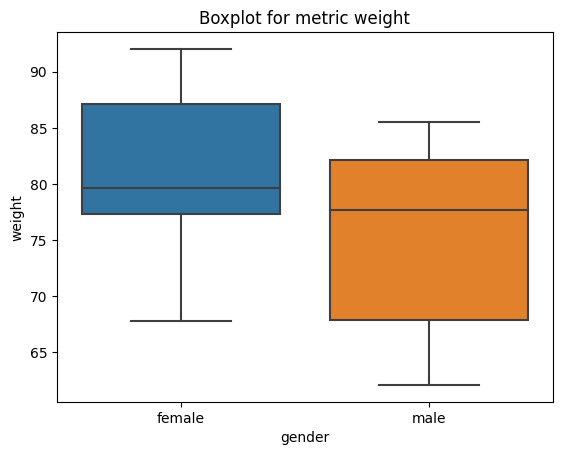
import seaborn as sns
import matplotlib.pyplot as plt

# obtain plots for our list
for i in list_num:
    sns.boxplot(x="gender", y=i, data=df)
    plt.title("Boxplot for metric " + i)
    plt.show()

Sorting

Sorting by values:

df.sort_values(by="height")

	name	id	height	average_height_parents	gender	number	height_m	weight	bmi	date
0	Stefanie	1	162	161.5	female	42	1.62	74.98	28.57	2023-03-21
1	Peter	2	163	163.5	male	42	1.63	62.06	23.36	2023-03-21
2	Stefanie	3	163	163.2	female	42	1.63	77.19	29.05	2023-03-21
3	Manuela	4	164	165.1	female	42	1.64	85.35	31.73	2023-03-21
4	Simon	5	164	163.2	male	42	1.64	72.68	27.02	2023-03-21
5	Sophia	6	164	164.4	female	42	1.64	67.78	25.20	2023-03-21
6	Ellen	7	164	164.0	female	42	1.64	81.99	30.48	2023-03-21
12	Fin	13	165	165.5	male	42	1.65	85.48	31.40	2023-03-21
11	Mila	12	165	167.4	female	42	1.65	79.65	29.26	2023-03-21
10	Lena	11	165	166.3	female	42	1.65	89.79	32.98	2023-03-21
9	Marie	10	165	165.1	female	42	1.65	78.47	28.82	2023-03-21
8	Lina	9	165	165.2	female	42	1.65	92.04	33.81	2023-03-21
7	Emilia	8	165	165.2	female	42	1.65	77.37	28.42	2023-03-21
13	Eric	14	166	166.2	male	42	1.66	83.14	30.17	2023-03-21
14	Pia	15	166	166.1	female	42	1.66	88.83	32.24	2023-03-21
15	Marc	16	166	166.5	male	42	1.66	82.14	29.81	2023-03-21
16	Ralph	17	166	166.6	male	42	1.66	63.43	23.02	2023-03-21
17	Tom	18	167	166.2	male	42	1.67	67.86	24.33	2023-03-21
18	Steven	19	167	167.3	male	42	1.67	80.69	28.93	2023-03-21
19	Emanuel	20	168	168.5	male	42	1.68	77.68	27.52	2023-03-21

Selection

Getting []

Selecting a single column (equivalent to df.height):

df["height"]

0     162
1     163
2     163
3     164
4     164
5     164
6     164
7     165
8     165
9     165
10    165
11    165
12    165
13    166
14    166
15    166
16    166
17    167
18    167
19    168
Name: height, dtype: int64

Selecting via [], which slices the rows (endpoint is not included).

df[0:1]

	name	id	height	average_height_parents	gender	number	height_m	weight	bmi	date
0	Stefanie	1	162	161.5	female	42	1.62	74.98	28.57	2023-03-21

By label .loc

The .loc attribute is the primary access method. The following are valid inputs:

For getting a cross section using a label:

df.loc[[0]]

	name	id	height	average_height_parents	gender	number	height_m	weight	bmi	date
0	Stefanie	1	162	161.5	female	42	1.62	74.98	28.57	2023-03-21

Selecting on a multi-axis by label:

df.loc[ : , ["name", "height"]]

	name	height
0	Stefanie	162
1	Peter	163
2	Stefanie	163
3	Manuela	164
4	Simon	164
5	Sophia	164
6	Ellen	164
7	Emilia	165
8	Lina	165
9	Marie	165
10	Lena	165
11	Mila	165
12	Fin	165
13	Eric	166
14	Pia	166
15	Marc	166
16	Ralph	166
17	Tom	167
18	Steven	167
19	Emanuel	168

Showing label slicing, both endpoints are included:

df.loc[0:1, ["name", "height"]]

	name	height
0	Stefanie	162
1	Peter	163

Reduction in the dimensions of the returned object:

df.loc[0, ["name", "height"]]

name      Stefanie
height         162
Name: 0, dtype: object

For getting a scalar value:

df.loc[[0], "height"]

0    162
Name: height, dtype: int64

By position .iloc

pandas provides a suite of methods in order to get purely integer based indexing. Here, the .iloc attribute is the primary access method.

df.iloc[0]

name                        Stefanie
id                                 1
height                           162
average_height_parents         161.5
gender                        female
number                            42
height_m                        1.62
weight                         74.98
bmi                            28.57
date                      2023-03-21
Name: 0, dtype: object

By integer slices:

df.iloc[0:2, 0:2]

	name	id
0	Stefanie	1
1	Peter	2

By lists of integer position locations:

df.iloc[[0, 2], [0, 2]]

	name	height
0	Stefanie	162
2	Stefanie	163

For slicing rows explicitly:

df.iloc[1:3, :]

	name	id	height	average_height_parents	gender	number	height_m	weight	bmi	date
1	Peter	2	163	163.5	male	42	1.63	62.06	23.36	2023-03-21
2	Stefanie	3	163	163.2	female	42	1.63	77.19	29.05	2023-03-21

For slicing columns explicitly:

df.iloc[:, 1:3]

	id	height
0	1	162
1	2	163
2	3	163
3	4	164
4	5	164
5	6	164
6	7	164
7	8	165
8	9	165
9	10	165
10	11	165
11	12	165
12	13	165
13	14	166
14	15	166
15	16	166
16	17	166
17	18	167
18	19	167
19	20	168

For getting a value explicitly:

df.iloc[0, 0]

'Stefanie'

Filter (boolean indexing)

Using a single column’s values to select data.

df[df["height"] > 180]

	name	id	height	average_height_parents	gender	number	height_m	weight	bmi	date

Using the isin() method for filtering:

df[df["name"].isin(["Tom", "Lisa"])]

	name	id	height	average_height_parents	gender	number	height_m	weight	bmi	date
17	Tom	18	167	166.2	male	42	1.67	67.86	24.33	2023-03-21

Grouping

By “group by” we are referring to a process involving one or more of the following steps:

• Splitting the data into groups based on some criteria

• Applying a function to each group independently

• Combining the results into a data structure

Grouping and then applying the mean() function to the resulting groups.

df.groupby("gender").mean().T

/tmp/ipykernel_1821/2544976795.py:1: FutureWarning: The default value of numeric_only in DataFrameGroupBy.mean is deprecated. In a future version, numeric_only will default to False. Either specify numeric_only or select only columns which should be valid for the function.
  df.groupby("gender").mean().T

gender	female	male
height	164.363636	165.777778
average_height_parents	164.863636	165.944444
number	42.000000	42.000000
height_m	1.643636	1.657778
weight	81.221818	75.017778
bmi	30.050909	27.284444

Segment data into bins

Use the function cut when you need to segment and sort data values into bins. This function is also useful for going from a continuous variable to a categorical variable.

In our example, we create a body mass index category. The standard weight status categories associated with BMI ranges for adults are shown in the following table:

BMI	Weight Status
Below 18.5	Underweight
18.5 - 24.9	Normal or Healthy Weight
25.0 - 29.9	Overweight
30.0 and Above	Obese

Source: U.S. Department of Health & Human Services

In our function, we discretize the variable bmi into four bins according to the table above:

• The bins [0, 18.5, 25, 30, float(‘inf’)] indicate (0,18.5], (18.5,25], (25,30], (30, float(‘inf))

• float('inf') is used for setting variable with an infinitely large value

df['bmi_category'] = pd.cut(df['bmi'], 
                            bins=[0, 18.5, 25, 30, float('inf')], 
                            labels=['underweight', 'normal', 'overweight', "obese"])

df['bmi_category']

0     overweight
1         normal
2     overweight
3          obese
4     overweight
5     overweight
6          obese
7     overweight
8          obese
9     overweight
10         obese
11    overweight
12         obese
13         obese
14         obese
15    overweight
16        normal
17        normal
18    overweight
19    overweight
Name: bmi_category, dtype: category
Categories (4, object): ['underweight' < 'normal' < 'overweight' < 'obese']