Data
Contents
Data
Data ingestion
There are various options how to store and ingest your data but we won’t go into the details of data engineering in this tutorial. However, if you want to learn more about topics like:
the basics of big data (Hadoop ecosystem and Spark),
relational and NoSQL databases,
how to set up a PostgreSQL and MySQL database,
examples of different data architectures and
components of machine learning operations (MLOps),
review this online book:
Jupyter Book
Prepare environment
In a real world data science project you would usually use a cloud environment (e.g. in Microsoft Azure, Google Cloud or Amazon AWS) to perform your data science project. However, for our course purposes, a local machine is fine. Here some steps to prepare your machine:
create a new folder (e.g.,
datascience) on your machine (which is not synchronized with a cloud service like Apple’s iCloud or Microsoft’s OneDrive)open a terminal where you can use
condaandcd(change directory) into your newly created folder:
cd datascience
use “cookiecutter” to create a data science folder structure (see this site for more details).
In your terminal:
cookiecutter -c v1 https://github.com/drivendata/cookiecutter-data-science
Connect your local folder with GitHub (visit this site for more information about GitHub).
Import data
The next step is to import the data. This means that you take data stored in a file, a relational database, a NoSQL database or data lakehouse and load it into Python. In our examples, we often use readr from the tidyverse and store it as df (short for DataFrame):
library(tidyverse)

path <- "path_to_data"

df <- read_csv(path)
Data structure
Next, we get a first impression of the data structure:
Take a look at the observations of your data:
df
View a description of the data, in particular the total number of rows and each attribute’s type:
glimpse(df)
The package visdat helps us to explore the data class structure visually:
library(visdat)

vis_dat(df)
Data corrections
Despite the fact that it would be easiest to preprocess your data right away with the tidyverse, we only take care of the most problematic errors (like the occurence of strings in data columns or wrong data formats). We only perform absolutely necessary data preprocessing because processing your data before passing it to packages like tidymodels - the tidymodels framework is a collection of packages for modeling and machine learning using tidyverse principles - might be problematic for one of the following reasons (scikit learn developers):
Incorporating statistics from data which later becomes our test data into the preprocessors makes cross-validation scores unreliable (known as data leakage), for example in the case of scalers (like z transformation) or imputing missing values.
You may want to include the parameters of the preprocessors in a parameter search (for hyperparameter tuning).
Later we will see that tidymodels recipes’s helps performing different transformations for different columns of the data within a data preprocessing pipeline that is safe from data leakage and that can be parametrized. To each column, a different transformation can be applied, such as preprocessing or a specific feature extraction method.
Note
As a general rule, we only take care of data errors which can be fixed without the risk of data leakage and which we don’t want to include as data preprocessing steps in a pipeline.
Example of data type transformation of one variable:
# convert to numeric
df <-
  df %>%
  mutate(
    foo = as.numeric(foo)
  )
Example of data type transformation:
# convert all character variables to factors
df <-
  df %>%
  mutate(across(where(is.character), as.factor))
Important note: Only use (across(where(is.character), as.factor) if you are certain that all remaining character variables are actually of type character (and not numeric variables which are falsely stored as type character).
Creation of new variables
During the creation of your plan, you maybe gained knowledge about possible ways to derive new variables from already existing columns in your dataset (e.g. through simple variable combinations). If this is the case, now would be a good time to create these variables.
dplyr offers multiple ways to derive new columns from existing columns (see this dplyr tutorial for more examples). Note that you create a new column by assigning the output to the DataFrame with the usage uf mutate and that operations are element-wise (i.e., no need to loop over rows):
df <-
    df %>%
 mutate(
  my_new_feature = feature_1 / feature_2,
  my_newest_feature = (feature_1 + feature_2) / 2
 )
Variable lists
We often need specific variables for exploratory data analysis as well as data preprocessing steps. We can use pandas to create specific lists (provided all columns are stored in the correct data format):
# list of all numerical data

list_num <-
  df %>%
  select(where(is.numeric)) %>%
  names()


# list of all categorical data
list_cat <-
  df %>%
  select(!where(is.numeric)) %>%
  names()
Furthermore, we prepare our data for the following processes of data splitting and building of data pipelines. Note that we use foo as placeholder for our outcome variable:
# define outcome variable as y_label
y_label <– 'foo'

# select feature names
features <-
  df %>%
  select(-all_of(y_label)) %>%
  names()

# create feature data for data splitting
X <-
  df %>%
  select(all_of(features))

# list of numeric feature names
feat_num <-
  X %>%
  select(where(is.numeric)) %>%
  names()

# list of categorical feature names
feat_cat <-
  X %>%
  select(!where(is.numeric)) %>%
  names()

# create response for data splitting
y <-
  df %>%
  select(all_of(y_label))
Data splitting
Before you start analyzing your data, it is a good idea to split your data into a training and test set [Géron, 2019]. We do this because this is the only way to know how well a model will generalize to new cases. Furthermore, we will perform exploratory data analysis only on the training data so we don’t use insights from the test data during the model building process.
Training, evaluation and test set
The error rate on new cases is called the generalization error (or out-of-sample error), and by evaluating our model on the test set, we get an estimate of this error. This value tells you how well your model will perform on instances it has never seen before. If the training error is low (i.e., your model makes few mistakes on the training set) but the generalization error is high, it means that your model is overfitting the training data.
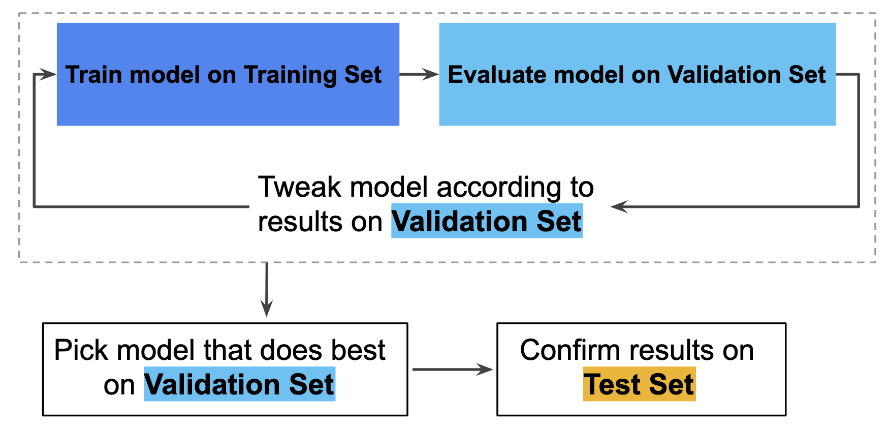
Note that if we want to evaluate different settings (“hyperparameters”) for models, such as the alpha in Lasso, there is still a risk of overfitting on the test set because the parameters can be tweaked until the model performs optimally (skicit learn developers). This way, knowledge about the test set can “leak” into the model and evaluation metrics no longer report on generalization performance. To solve this problem, yet another part of the dataset can be held out as a so-called “validation set”: training proceeds on the training set, after which evaluation is done on the validation set, and when the experiment seems to be successful, final evaluation can be done on the test set.
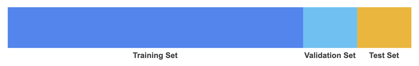
Hence, you can greatly reduce your chances of overfitting by partitioning the data set into the three subsets shown in the following figure (Google Developers):
In this workflow, you pick the model that does best on the validation set and double-check that model against the test set (Google Developers):
However, by partitioning the available data into three sets, we drastically reduce the number of samples which can be used for learning the model, and the results can depend on a particular random choice for the pair of (train, validation) sets (skicit learn developers). A solution to this problem is a procedure called cross-validation (CV for short). A test set should still be held out for final evaluation, but the validation set is no longer needed when doing CV. In the basic approach, called k-fold CV, the training set is split into k smaller sets.
Train and test split
We typically use rsample’s initial_split to perform data splitting and use set.seed() to make this notebook’s output identical at every run (we arbitrarily set the number to 42 but you can choose any other number):
library(rsample)

# Fix the random numbers by setting the seed
# This enables the analysis to be reproducible
set.seed(42)

# Put 3/4 of the data into the training set
data_split <- initial_split(df,
                           prop = 3/4,
                           strata = y_label,
                           breaks = 4)

# Create dataframes for the two sets:
train_data <- training(data_split)
test_data <- testing(data_split)
prop: The proportion of data to be retained for modeling/analysis.strata: A variable in data (single character or name) used to conduct stratified sampling. When not NULL, each resample is created within the stratification variable. Numeric strata are binned into quartiles.breaks: A single number giving the number of bins desired to stratify a numeric stratification variable.
We can now create a validation set, which we use during modeling:
library(tidymodels)

set.seed(42)

cv_folds <-
  vfold_cv(train_data,
           v=5,
           strata = y_label,
           breaks = 4)
Data exploration set
We make a copy of the training data since we don’t want to alter our data during data exploration. We will use this data for our exploratory data analysis:
df_train <- train_data
Analyze data
The goal of this phase is to understand the training data. In particular, exploratory data analysis (EDA) is used to understand important predictor characteristics.
Note
The interactive website From Data to Viz leads you to the most appropriate graph for your data.
Good visualisations will show you things that you did not expect, or raise new questions about the data [Wickham and Grolemund, 2016]: A good visualisation might also hint that you’re asking the wrong question, or you need to collect different data.
Furthermore, we want to understand if there are any challenges associated with the data that can be discovered prior to modeling.
We can obtain a data summary of all numerical and categorical attributes of our training data by using a function from the package skimr:
library(skimr)

skim(df_train)
To learn more about data visualization in R, visit this resources:
Note that in the next section, we will use lists created in Variable lists for some of the steps shown below.
Categorical data
For categorical data we check the levels and their uniqueness (e.g. with bar plots):
for (i in feat_cat){

  p <- ggplot(df_train, aes_string(x=i)) +
  geom_bar()

  plot(p)
  }
To learn more about categorical data visualizations, visit the following book:
Resources
Numerical grouped by categorical
We can also investigate our numerical data grouped by a categorical variable. This time, we use the purrr package:
library(purrr)

df_train %>%
  split(feat_cat) %>%
  map(summary)
Alternative approach for one specific categorical variable:
# median
df_train %>%
  group_by(my_categorical_variable) %>%
  summarise(across(feat_num, median, na.rm = TRUE))

# mean
df_train %>%
  group_by(my_categorical_variable) %>%
  summarise(across(feat_num, mean, na.rm = TRUE))

# standard deviation
df_train %>%
  group_by(my_categorical_variable) %>%
  summarise(across(feat_num, sd, na.rm = TRUE))
To learn more about data visualizations, visit the following site:
Numerical data
A quick way to get an overview of the type of data you are dealing with is to plot a histogram for each numerical attribute. A histogram shows the number of instances (on the vertical axis) that have a given value range (on the horizontal axis). You can either plot this one attribute at a time, or you can use ggscatmat from the package GGally on the whole dataset (as shown in the following code example), and it will plot a histogram for each numerical attribute as well as correlation coefficients (Pearson is the default). We just select the most promising variabels for our plot:
library(GGally)

df_train %>%
  select(feat_num) %>%
  ggscatmat(alpha = 0.2)
To learn more about data visualizations, visit the following site:
Resources
Relationships
Detect the relationship between each predictor and the response:
library(GGally)

df_train %>%
  ggpairs()
To obtain the correlations of our numerical data, we can use the function vis_cor from the visdat package. We use Spearman’s correlation coefficient since this measure is more insensitive to outliers than Pearson’s correlation coefficient:
library(visdat)

df_train %>%
  select(where(is.numeric)) %>% # only select numerical data
  vis_cor(cor_method = "spearman", na_action = "pairwise.complete.obs")
Now we take a closer look at the correlation coefficients with the package corrr.
# calculate all correlations
cor_res <-
  df_train %>%
  select(where(is.numeric)) %>%
  correlate(method = "spearman", use = "pairwise.complete.obs")

# show correlations
cor_res %>%
  select(term, y_label) %>%
  filter(!is.na(y_label)) %>% # focus on dependent variable
  arrange(y_label) %>% # sort values
  fashion() # print tidy correlations
The package tidymodels also provides a step_corr which creates a specification of a recipe step that will potentially remove variables that have large absolute correlations with other variables.
Define schema
Usually it is a good idea to define some sort of schema that describes the expected properties of the data. Some of these properties are (TensorFlow):
which features are expected to be present
their type
the number of values for a feature in each example
the presence of each feature across all examples
the expected domains of features.
Tidymodels provides multiple functions to check data before it get’s passed over to algorithms.
We don’t cover this topic in detail here but if you want to learn more about schemas, check out the following resources:
Anomaly detection
Next, we need to identify missing values and anomalies in the data (with respect to a given schema).
Note that we just gain insights and don’t perform any data preprocessing during the phase of anomaly detection. We only need to decide how to deal with the issues we detect. All data transformations will be performed during feature engineering (with tidymodels pipelines).
Missing values
We check the degree of missingness within each predictor in the original dataframe to avoid code duplication (otherwise we first would perform all checks on df_train and afterwards on df_test).
Note
We use the original dataframe df to check for missing values
Missing data can be viewed with the function vis_miss from the package visdat. We arrange the data by columns with most missingness:
# missing values will be displayed in black
vis_miss(df, sort_miss = TRUE)
# absolute number of missing values
is.na(df) %>%
    colSums()
We cover the topic of how to handle missing data in the section about preprocessing pipelines.
Outlier and novelty detection
Many applications require being able to decide whether a new observation belongs to the same distribution as existing observations (it is an inlier), or should be considered as different (it is an outlier). Two important distinctions must be made (scikit-learn developers):
outlier detection: The training data contains outliers which are defined as observations that are far from the others. Outlier detection estimators thus try to fit the regions where the training data is the most concentrated, ignoring the deviant observations.
novelty detection: The training data is not polluted by outliers and we are interested in detecting whether a new observation is an outlier. In this context an outlier is also called a novelty.
Again, we first use data exploration to gain insights about unusual cases. In addition to the plots covered in (histograms are especially relevant), we can use boxplots for our numerical data:
# boxplots
for (i in feat_cat){

    p <- ggplot(df_train, aes_string(x=i, y=y_label)) +
      geom_boxplot(fill="steelblue")

    plot(p)
  }
To investigate categorical data we can use the same methods as described in Categorical data.
Feature engineering
“Applied machine learning is basically feature engineering” Andrew Ng
The understanding gained in data analysis is now used for data preprocessing (e.g., encode categorical data, fix missing values and outliers) and feature engineering.
Feature engineering is the process of using domain knowledge to extract meaningful features (attributes) from raw data. The goal of this process is to create new features which improve the predictions from our model and my include steps like [Kuhn and Johnson, 2019]:
Feature transformation (transform features)
Feature extraction (reduce the number of features by combining existing features)
Feature creation (make new features)
Note that the usage of data pipelines is considered best practice to help avoid leaking statistics from your test data into the trained model during data preprocessing and feature engineering. Therefore, we first take a look at pipelines.
Note
The topic of feature selection is part of the model building process and will be covered in the modeling phase.
Pipelines
The R package tidymodels provides a library for data preprocessing and feature engineering:
Pipelines
Tidymodel’s recipes documentation
Feature transformation
Typically, we need to perform feature transformations because predictors may [Kuhn and Johnson, 2019]:
have missing values
contain a small number of extreme values (outliers)
be on vastly different scales
need to be numeric instead of categorical
follow a skewed distribution where a small proportion of samples are orders of magnitude larger than the majority of the data (i.e., skewness).
be censored on the low and/or high end of the range.
Fix missing values
If we find missing cases in our data, we need to decide how to deal with them. For example, we could:
Get rid of the corresponding observations.
Get rid of the whole attribute.
Impute with some other value (zero, the mean, the median, etc.).
Usually we will include an imputation of missing values in our pipeline.
Fix outliers
There are various options of how to fix outliers. However, tidymodels currently does not provide sophisticated solutions to handle outliers. At the moment, there are only experimental solutions of 3-rd party packages like tidy.outliers available.
Feature scaling
Feature scaling is a method used to change raw feature vectors into a representation that is more suitable for learning algorithms.
Note
Scaling the target values is generally not required.
Types
Most learning algorithms benefit from standardization (normalization) of the data set since they don’t perform well when the input numerical attributes have very different scales (think of different measurment units like cm and m). For instance, many elements used in the objective function of a learning algorithm (such as the RBF kernel of Support Vector Machines or the l1 and l2 regularizers of linear models) assume that all features are centered around zero and have variance in the same order (an exception are decision tree-based estimators since they are robust to arbitrary scaling of the data).
In our projects, we usually use standardization to scale our features: Standardization centers the data by removing the mean value of each feature, then scale it by dividing features by their standard deviation. This leads to a standard normally Gaussian distribution with zero mean and unit variance.
Tidymodels provides a transformer called step_normalize for this:
Note that this process cannot guarantee balanced feature scales in the presence of outliers.
Encode categorical features
Usually algorithms prefer to work with numbers, so we need to convert categorial variables from text to numbers.
Tidymodels provides a step_dummy function to convert categorical values into one-hot vectors (one-hot encoding) which we will use in our data preprocessing pipeline.
Feature extraction
Features may contain relevant but overly redundant information. That is, the information collected could be more effectively and efficiently represented with a smaller, consolidated number of new predictors while still preserving or enhancing the new predictors’ relationship with the response [Kuhn and Johnson, 2019]. In that case, feature extraction can be achieved by simply using the ratio of two predictors or with the help of more complex methods like pricipal component analysis.
If your number of features is high, it may be useful to reduce it with an unsupervised step prior to supervised steps. You can reduce features with different unsupervised and supervised dimensionality reduction methods:
Custom feature operations
Although tidymodels provides many useful recipes, eventually you may need to write your own functions for tasks such as custom data cleaning procedures or feature engineering.
You find an example of how to build your own solutions here.
Final data pipeline
In this final step, we will build a typical data preprocessing pipeline using some of the functions covered in the previous sections.
Note
We use features created in Variable lists for some of the steps shown below
library(tidymodels)

df_rec <-
  recipe(your_y_label ~ ., data = train_data) %>%
  step_impute_median(all_numeric(), -all_outcomes()) %>%
  step_impute_mode(all_nominal_predictors()) %>%
  step_normalize(all_numeric(), -all_outcomes()) %>%
  step_dummy(all_nominal_predictors()) %>%
  step_corr(all_predictors(), threshold = 0.7, method = "spearman")
In the following model building phase (see Model), section “Train and evaluate”, we can easily combine our full pipline with scikit-learn algorithms.