Model#

Once our features have been preprocessed in a format ready for modeling (see Data), they can be used in the model selection process.

Note

The type of data preprocessing is dependent on the type of model being fit. Kuhn and Silge [2021] provide recommendations for baseline levels of preprocessing that are needed for various model functions (see this table).

The following Jupyter Books provide information about different regression and classification models:

Jupyter Book

Next, we discuss some important model selection topics like

Model selection
best fitting model
mean squared error
bias-variance trade off.

Resources

In the next sections, we’ll discuss the process of model building in detail.

Select model#

One of the hardest parts during the data science lifecycle can be finding the right model for the job since different types of models are better suited for different types of data and different problems. For some datasets the best model could be a linear model, while for other datasets it is a random forest or neural network. There is no model that is a priori guaranteed to work better. This fact is known as the “No Free Lunch (NFL) theorem” [Wolpert, 1996].

Resources

Download slides

Some of the most common models are (take a look at the Jupyter Books Regression and Classification for more details):

Linear and Polynomial Regression,
Logistic Regression,
k-Nearest Neighbors,
Support Vector Machines,
Decision Trees,
Random Forests,
Neural Networks and
Ensemble methods like Gradient Boosted Decision Trees (GBDT).

A model ensemble, where the predictions of multiple single learners are aggregated together to make one prediction, can produce a high-performance final model. The most popular methods for creating ensemble models in scikit-learn are:

Bootstrap aggregating, also called bagging (from bootstrap aggregating)
random forest
Boosting: AdaBoost and Gradient Tree Boosting

Each of these methods combines the predictions from multiple versions of the same type of model (e.g., classifications trees).

Note that the only way to know for sure which model is best would be to evaluate them all [Géron, 2019]. Since this is often not possible, in practice you make some assumptions about the data and evaluate only a few reasonable models. For example, for simple tasks you may evaluate linear models with various levels of regularization as well as some ensemble methods like Gradient Boosted Decision Trees (GBDT). For very complex problems, you may evaluate various deep neural networks.

The following flowchart was provided by scikit-learn developers to give users a bit of a rough guide on how to approach problems with regard to which models to try on your data:

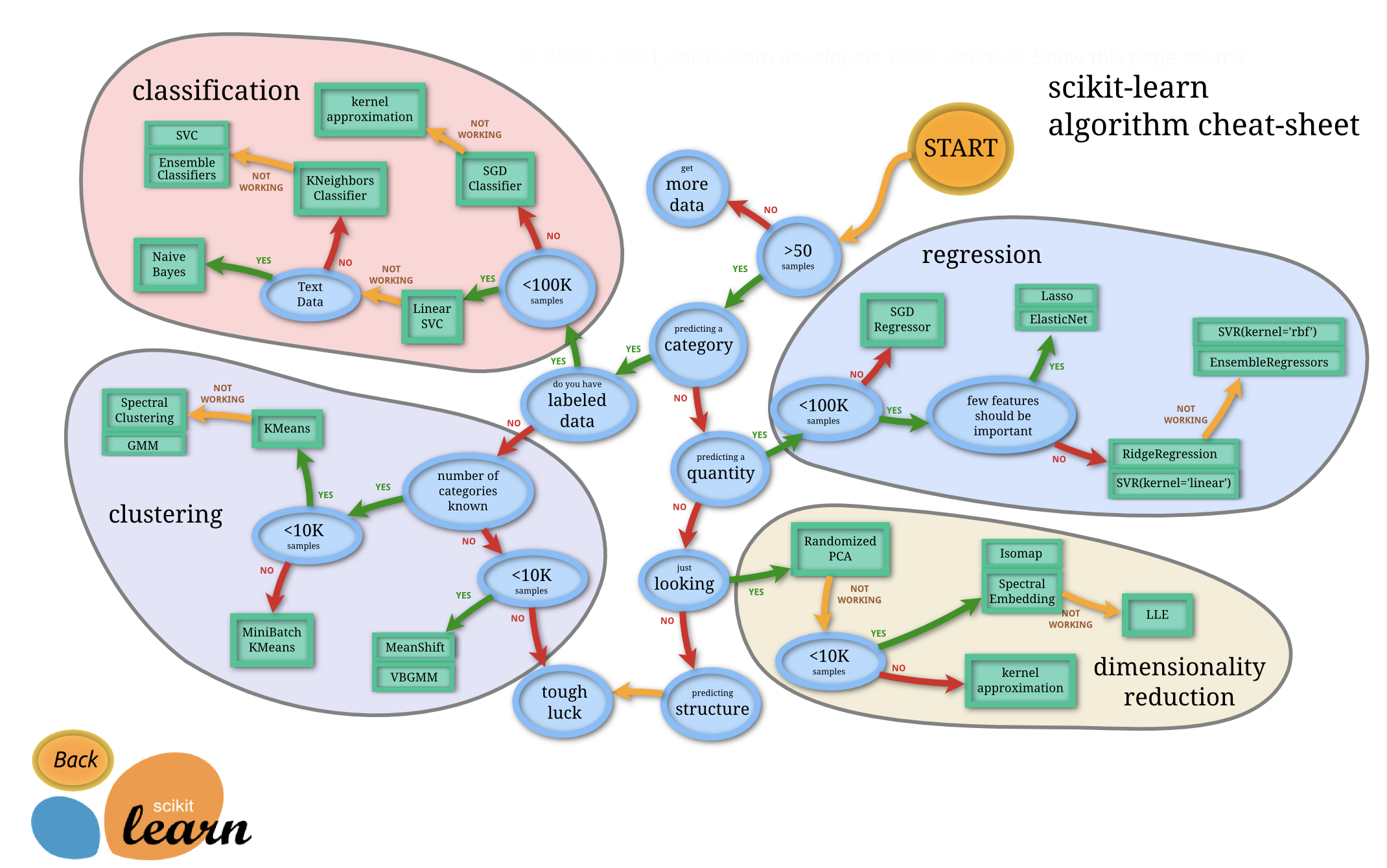
Visit this site to interact with the flowchart.

Train and evaluate#

In the first phase of the model building process, a variety of initial models are generated and their performance is compared during model evaluation. As a part of this process, we also need to decide which features we want to include in our model (“feature selection”). Therefore, let’s first take a look at the topic of feature selection.

Feature selection#

There are a number of different strategies for feature selection that can be applied and some of them are performed simultaneously with model building.

Note

Feature selection is the process of selecting a subset of relevant features (variables, predictors) for our model.

If you want to learn more about feature selection methods, review the following content:

Jupyter Book

Feature Selection

Training#

Now we can use the pipeline we created in Data (see last section) and combine it with scikit-learn algorithms of our choice:

from sklearn.linear_model import LinearRegression

# Use pipeline with linear regression model
lm_pipe = Pipeline(steps=[
            ('full_pipeline', full_pipeline),
            ('lm', LinearRegression())
                         ])

# Show pipeline as diagram
set_config(display="diagram")

# Fit model
lm_pipe.fit(X_train, y_train)

# Obtain model coefficients
lm_pipe.named_steps['lm'].coef_

Evaluation#

In model evaluation, we mainly assess the model’s performance metrics (using an evaluation set) and examine residual plots (see this example for linear regression diagnostics) to understand how well the models work. Our first goal in this process is to shortlist a few (two to five) promising models.

Scikit-learn provides an extensive list of possible metrics to quantify the quality of model predictions:

Metrics

Metrics and scoring: quantifying the quality of predictions

from sklearn.metrics import r2_score
from sklearn.metrics import mean_squared_error
from sklearn.metrics import mean_absolute_error


# obtain predictions for training data
y_pred = lm_pipe.predict(X_train)

# R squared
r2_score(y_train, y_pred) 

# MSE
mean_squared_error(y_train, y_pred)

# RMSE
mean_squared_error(y_train, y_pred, squared=False)

# MAE
mean_absolute_error(y_train, y_pred)

Show residual plot:

import seaborn as sns

sns.residplot(x=y_pred, y=y_train, scatter_kws={"s": 80});

Tuning#

After we identified a shortlist of promising models, it usually makes sense to tune the hyper-paramters of our models.

Note

Hyper-parameters are parameters that are not directly learnt within algorithms.

In scikit-learn, hyper-paramters are passed as arguments to the algorithm like “alpha” for Lasso or “K” for the number of neighbors in a K-nearest neighbors model.

Instead of trying to find good hyper-paramters manually, it is recommended to search the hyper-parameter space for the best cross validation score using one of the two generic approaches provided in scikit-learn:

for given values, GridSearchCV exhaustively considers all parameter combinations.
RandomizedSearchCV can sample a given number of candidates from a parameter space with a specified distribution.

Tuning

Tuning the hyper-parameters of an estimator

The GridSearchCV approach is fine when you are exploring relatively few combinations, but when the hyperparameter search space is large, it is often preferable to use RandomizedSearchCV instead [Géron, 2019]. Both methods use cross-validation (CV) to evaluate combinations of hyperparameter values.

Next, we take a look at an example of hyperparameter tuning with a skicit-learn pipeline (scikit-learn developers) for a classification problem (we use the dataset digits) with logistic regression. In particular, we define a pipeline to search for the best combination of PCA truncation and classifier regularization:

import numpy as np
from sklearn import datasets
from sklearn.decomposition import PCA
from sklearn.linear_model import LogisticRegression
from sklearn.pipeline import Pipeline
from sklearn.model_selection import GridSearchCV
from sklearn.preprocessing import StandardScaler

# Pipeline
pipe = Pipeline(steps=[
    ("scaler", StandardScaler()), 
    ("pca", PCA()), 
    ("logistic", LogisticRegression(max_iter=10000, tol=0.1))])

# Data
X_digits, y_digits = datasets.load_digits(return_X_y=True)

# Parameters of pipelines can be set using ‘__’ separated parameter names:
param_grid = {
    "pca__n_components": [5, 15, 30, 45, 60],
    "logistic__C": np.logspace(-4, 4, 4),
}

# Gridsearch
search = GridSearchCV(pipe, param_grid, n_jobs=2)
search.fit(X_digits, y_digits)

# Show results
print("Best parameter (CV score=%0.3f):" % search.best_score_)
print(search.best_params_)

pca__n_components: Number of components to keep
logistic__c: Each of the values in Cs describes the inverse of regularization strength. If Cs is as an int, then a grid of Cs values are chosen in a logarithmic scale between 1e-4 and 1e4. Smaller values specify stronger regularization.

Voting and stacking#

It often makes sense to combine different models since the group (“ensemble”) will usually perform better than the best individual model, especially if the individual models make very different types of errors.

Note

Voting can be useful for a set of equally well performing models in order to balance out their individual weaknesses.

Model voting combines the predictions for multiple models of any type and thereby creating an ensemble meta-estimator. scikit-learn provides voting methods for both classification (VotingClassifier) and regression (VotingRegressor):

In classification problems, the idea behind voting is to combine conceptually different machine learning classifiers and use a majority vote or the average predicted probabilities (soft vote) to predict the class labels.
In regression problems, we combine different machine learning regressors and return the average predicted values.

Voting regressor

Voting regressor example

Stacked generalization is a method for combining estimators to reduce their biases. Therefore, the predictions of each individual estimator are stacked together and used as input to a final estimator to compute the prediction. This final estimator is trained through cross-validation.

Note

Model stacking is an ensembling method that takes the outputs of many models and combines them to generate a new model that generates predictions informed by each of its members.

In scikit-learn, the StackingClassifier and StackingRegressor provide such strategies which can be applied to classification and regression problems.

To learn more about the concept of stacking, visit the documentation of stacks, a R package for model stacking.

Evaluate best model#

After we tuned hyper-parameters and/or performed voting/stacking, we evaluate the best model (system) and their errors in more detail.

In particular, we take a look at the specific errors that our model (system) makes, and try to understand why it makes them and what could fix the problem - like adding extra features or getting rid of uninformative ones, cleaning up outliers, etc. [Géron, 2019]. If possible, we also display the importance scores of our predictors (e.g. using scikit-learn’s permutation feature importance). With this information, we may want to try dropping some of the less useful features to make sure our model generalizes well.

For example, you could assess possible reasons for the 10 wrongest model predictions:

# create dataframe
df_error = pd.DataFrame(
    { "y": y_train,
      "y_pred": y_pred,
      "error": y_pred - y_train
    })

# sort by error, select top 10 and get index
error_index = df_error.sort_values(by=['error']).nlargest(10, 'error').index

# show corresponding data observations
df.iloc[error_index]

After evaluating the model (system) for a while, we eventually have a system that performs sufficiently well.

Evaluate on test set#

Now is the time to evaluate the final model on the test set. If you did a lot of hyperparameter tuning, the performance will usually be slightly worse than what you measured using cross-validation - because your system ends up fine-tuned to perform well on the validation data and will likely not perform as well on unknown dataset [Géron, 2019].

y_pred = lm_pipe.predict(X_test)

print('MSE:', mean_squared_error(y_test, y_pred))

print('RMSE:', mean_squared_error(y_test, y_pred, squared=False))

It is important to note that we don’t change the model (system) anymore to make the numbers look good on the test set; the improvements would be unlikely to generalize to new data. Instead, we use the metrics for our final evaluation to make sure the model performs sufficiently well regarding our success metrics from the planning phase.

Data Science with Python

Model

Contents

Model#

Select model#

Train and evaluate#

Feature selection#

Training#

Evaluation#

Tuning#

Voting and stacking#

Evaluate best model#

Evaluate on test set#

Challenges#