Credit data

The credit data is a simulated data set containing information on ten thousand customers (taken from James et al. [2021]). The aim here is to use a classification model to predict which customers will default on their credit card debt (i.e., failure to repay a debt):

• default: A categorical variable with levels No and Yes indicating whether the customer defaulted on their debt

• student: A categorical variable with levels No and Yes indicating whether the customer is a student

• balance: The average balance that the customer has remaining on their credit card after making their monthly payment

• income: Income of customer

Import data

import pandas as pd

df = pd.read_csv('https://raw.githubusercontent.com/kirenz/classification/main/_static/data/Default.csv')

Inspect data

df

	default	student	balance	income
0	No	No	729.526495	44361.625074
1	No	Yes	817.180407	12106.134700
2	No	No	1073.549164	31767.138947
3	No	No	529.250605	35704.493935
4	No	No	785.655883	38463.495879
...	...	...	...	...
9995	No	No	711.555020	52992.378914
9996	No	No	757.962918	19660.721768
9997	No	No	845.411989	58636.156984
9998	No	No	1569.009053	36669.112365
9999	No	Yes	200.922183	16862.952321

10000 rows × 4 columns

df.info()

<class 'pandas.core.frame.DataFrame'>
RangeIndex: 10000 entries, 0 to 9999
Data columns (total 4 columns):
 #   Column   Non-Null Count  Dtype  
---  ------   --------------  -----  
 0   default  10000 non-null  object 
 1   student  10000 non-null  object 
 2   balance  10000 non-null  float64
 3   income   10000 non-null  float64
dtypes: float64(2), object(2)
memory usage: 312.6+ KB

# check for missing values
print(df.isnull().sum())

default    0
student    0
balance    0
income     0
dtype: int64

Data preparation

Categorical data

First, we convert categorical data into indicator variables:

dummies = pd.get_dummies(df[['default', 'student']], drop_first=True, dtype=float)
dummies.head(3)

	default_Yes	student_Yes
0	0.0	0.0
1	0.0	1.0
2	0.0	0.0

# combine data and drop original categorical variables
df = pd.concat([df, dummies], axis=1).drop(columns = ['default', 'student'])
df.head(3)

	balance	income	default_Yes	student_Yes
0	729.526495	44361.625074	0.0	0.0
1	817.180407	12106.134700	0.0	1.0
2	1073.549164	31767.138947	0.0	0.0

Label and features

Next, we create our y label and features:

y = df['default_Yes']
X = df.drop(columns = 'default_Yes')

Train test split

from sklearn.model_selection import train_test_split

X_train, X_test, y_train, y_test = train_test_split(X, y, test_size=0.3, random_state = 1)

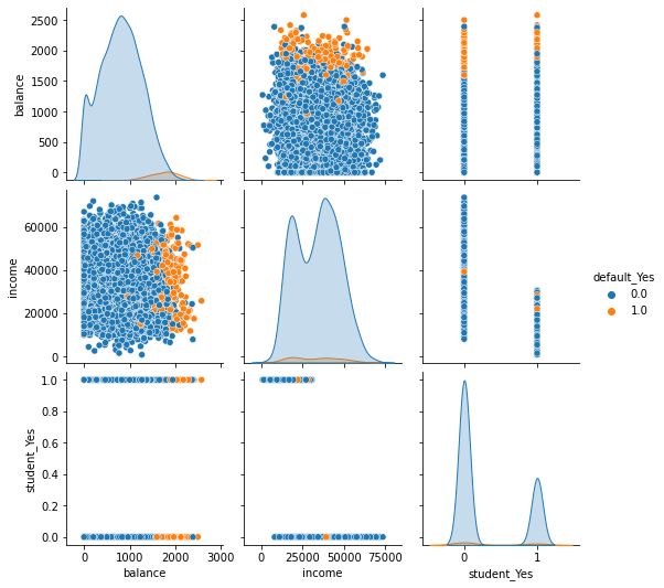
Data exploration

Create data for exploratory data analysis.

train_dataset = pd.DataFrame(X_train.copy())
train_dataset['default_Yes'] = pd.DataFrame(y_train)

import seaborn as sns

sns.pairplot(train_dataset, hue='default_Yes');