Online ads#

In this problem set we analyse the relationship between online ads and purchase behavior. In particular, we want to classify which online users are likely to purchase a certain product after being exposed to an online ad.

Setup#

import pandas as pd

import altair as alt
import seaborn as sns

from sklearn.model_selection import train_test_split
from sklearn.linear_model import LogisticRegressionCV

Data#

Import data#

df = pd.read_csv("https://raw.githubusercontent.com/kirenz/datasets/master/purchase.csv")

Data structure#

df

	Unnamed: 0	User ID	Gender	Age	EstimatedSalary	Purchased
0	1	15624510	Male	19	19000	0
1	2	15810944	Male	35	20000	0
2	3	15668575	Female	26	43000	0
3	4	15603246	Female	27	57000	0
4	5	15804002	Male	19	76000	0
...	...	...	...	...	...	...
395	396	15691863	Female	46	41000	1
396	397	15706071	Male	51	23000	1
397	398	15654296	Female	50	20000	1
398	399	15755018	Male	36	33000	0
399	400	15594041	Female	49	36000	1

400 rows × 6 columns

df.info()

<class 'pandas.core.frame.DataFrame'>
RangeIndex: 400 entries, 0 to 399
Data columns (total 6 columns):
 #   Column           Non-Null Count  Dtype 
---  ------           --------------  ----- 
 0   Unnamed: 0       400 non-null    int64 
 1   User ID          400 non-null    int64 
 2   Gender           400 non-null    object
 3   Age              400 non-null    int64 
 4   EstimatedSalary  400 non-null    int64 
 5   Purchased        400 non-null    int64 
dtypes: int64(5), object(1)
memory usage: 18.9+ KB

# inspect outcome variable
df['Purchased'].value_counts()

0    257
1    143
Name: Purchased, dtype: int64

Data corrections#

# change data format
df['Purchased'] = df['Purchased'].astype('category')

# make dummy variable
df['male'] = pd.get_dummies(df['Gender'], drop_first = True)

# drop irrelevant columns
df.drop(columns= ['Unnamed: 0', 'User ID', 'Gender'], inplace = True)

Variable lists#

# prepare data for scikit learn 
y_label = 'Purchased'

X = df.drop(columns=[y_label])
y = df[y_label]

Data split#

# make data split
X_train, X_test, y_train, y_test = train_test_split(X, y, test_size=0.3, random_state = 1)

Data exploration set#

# create new training dataset for data exploration
df_train = pd.DataFrame(X_train).copy()
df_train['Purchased'] = pd.DataFrame(y_train)

df_train

	Age	EstimatedSalary	male	Purchased
39	27	31000	0	0
167	35	71000	0	0
383	49	28000	1	1
221	35	91000	1	1
351	37	75000	1	0
...	...	...	...	...
255	52	90000	0	1
72	20	23000	0	0
396	51	23000	1	1
235	46	79000	1	1
37	30	49000	1	0

280 rows × 4 columns

Analyze data#

df_train.groupby(by=['Purchased']).describe().T

	Purchased	0	1
Age	count	185.000000	95.000000
	mean	32.621622	45.821053
	std	7.957603	8.756735
	min	18.000000	27.000000
	25%	27.000000	39.000000
	50%	33.000000	47.000000
	75%	38.000000	52.500000
	max	59.000000	60.000000
EstimatedSalary	count	185.000000	95.000000
	mean	58556.756757	89505.263158
	std	22429.073482	43284.038059
	min	15000.000000	20000.000000
	25%	43000.000000	43500.000000
	50%	60000.000000	97000.000000
	75%	75000.000000	130000.000000
	max	134000.000000	150000.000000
male	count	185.000000	95.000000
	mean	0.518919	0.452632
	std	0.500998	0.500392
	min	0.000000	0.000000
	25%	0.000000	0.000000
	50%	1.000000	0.000000
	75%	1.000000	1.000000
	max	1.000000	1.000000

Purchasers are (on average) _______ and earn a __________ estimated salary than non-purchasers.

Visualization of differences:

alt.Chart(df_train).mark_circle().encode(
    alt.X(alt.repeat("column"), type='quantitative'),
    alt.Y(alt.repeat("row"), type='quantitative'),
    alt.Color('Purchased:N'),
).properties(
    width=150,
    height=150
).repeat(
    row=['Age', 'EstimatedSalary', 'male'],
    column=['Age', 'EstimatedSalary', 'male']
).interactive()

Code for seaborn:

sns.pairplot(hue='Purchased', kind="reg", diag_kind="kde", data=df_train);

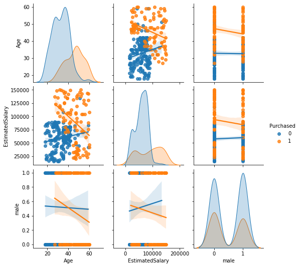
Inspect (linear) relationships between variables with correlation (pearson’s correlation coefficient)

df.corr().round(2)

	Age	EstimatedSalary	male
Age	1.00	0.16	-0.07
EstimatedSalary	0.16	1.00	-0.06
male	-0.07	-0.06	1.00

alt.Chart(df_train).mark_area(
    opacity=0.5,
    interpolate='step'
).encode(
    alt.X("Age:Q", bin=alt.Bin(maxbins=20)),
    alt.Y('count()', stack = None),
    alt.Color('Purchased:N'),
).properties(width=300)

Code for seaborn:

sns.histplot(hue="Purchased", x='Age', data=df_train);

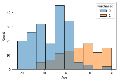
Purchasers seem to be _________ than non-purchaser.

alt.Chart(df_train).mark_boxplot(
    size=50,
    opacity=0.7
).encode(
    x='male:N',
    y=alt.Y('Age:Q', scale=alt.Scale(zero=True)),  
    color='Purchased:N'
).properties(width=300)

Code for seaborn

sns.boxplot(x="male", y="Age", hue="Purchased", data=df_train);

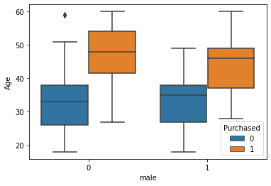
There are __________ differences regarding gender.

alt.Chart(df_train).mark_area(
    opacity=0.5,
    interpolate='step'
).encode(
    alt.X("EstimatedSalary:Q", bin=alt.Bin(maxbins=20)),
    alt.Y('count()', stack = None),
    alt.Color('Purchased:N'),
).properties(width=300)

Code for seaborn

sns.histplot(hue="Purchased", x='EstimatedSalary', data=df_train); 

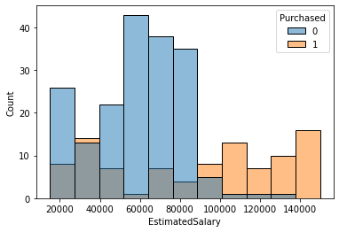
Purchaser earn a ______________ estimated salary.

alt.Chart(df_train).mark_boxplot(
    size=50,
    opacity=0.7
).encode(
    x='male:N',
    y=alt.Y('EstimatedSalary:Q', scale=alt.Scale(zero=True)),  
    color='Purchased:N'
).properties(width=300)

Code for seaborn

sns.boxplot(x="male", y="EstimatedSalary", hue="Purchased", data=df_train);

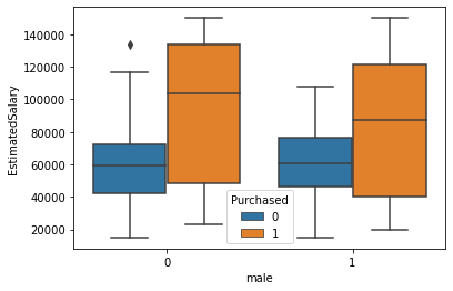
Insight: there are ___________ differences between males and females (regarding purchase behavior, age and estimated salary)

Select features#

# only select meaningful predictors

features_model = ['Age', 'EstimatedSalary']

X_train = X_train[features_model] 
X_test = X_test[features_model]

Model#

Select model#

Next, we will fit a logistic regression model with a L2 regularization (ridge regression). In particular, we use an estimator that has built-in cross-validation capabilities to automatically select the best hyper-parameter for our L2 regularization (see the documentation).

We only use our most promising predictor variables Age and EstimatedSalary for our model.

# model
clf = LogisticRegressionCV()

Training#

# fit model to data
clf.fit(X_train, y_train)

LogisticRegressionCV()

In a Jupyter environment, please rerun this cell to show the HTML representation or trust the notebook.
On GitHub, the HTML representation is unable to render, please try loading this page with nbviewer.org.

Coefficients#

clf.intercept_

array([-4.64629128])

clf.coef_

array([[7.57358038e-02, 1.72880947e-05]])

Classification metrics#

# Return the mean accuracy on the given test data and labels:
clf.score(X_test, y_test)

0.7833333333333333

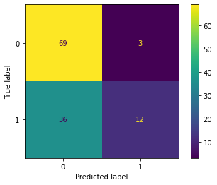
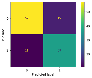
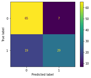
from sklearn.metrics import ConfusionMatrixDisplay

ConfusionMatrixDisplay.from_estimator(clf, X_test, y_test);

from sklearn.metrics import classification_report

y_pred = clf.predict(X_test)

print(classification_report(y_test, y_pred, target_names=['No', 'Yes']))

              precision    recall  f1-score   support

          No       0.77      0.90      0.83        72
         Yes       0.81      0.60      0.69        48

    accuracy                           0.78       120
   macro avg       0.79      0.75      0.76       120
weighted avg       0.79      0.78      0.78       120

The (unweighted) recall of our model is _____

The (unweighted) precision of our model is _____

ROC Curve#

from sklearn.metrics import RocCurveDisplay

RocCurveDisplay.from_estimator(clf, X_test, y_test) ;

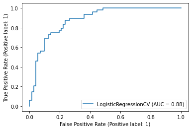
AUC Score#

from sklearn.metrics import roc_auc_score

y_score = clf.predict_proba(X_test)[:, 1]
roc_auc_score(y_test, y_score)

0.8842592592592593

Thresholds#

We use three different thresholds. Which threshold would you recommend if we want to maximize our F1-Score?

pred_proba = clf.predict_proba(X_test)

Threshold 0.4#

df_04 = pd.DataFrame({'y_pred': pred_proba[:,1] > .4})

ConfusionMatrixDisplay.from_predictions(y_test, df_04['y_pred']);

print(classification_report(y_test, df_04['y_pred']))

              precision    recall  f1-score   support

           0       0.84      0.79      0.81        72
           1       0.71      0.77      0.74        48

    accuracy                           0.78       120
   macro avg       0.77      0.78      0.78       120
weighted avg       0.79      0.78      0.78       120

Threshold 0.5#

df_05 = pd.DataFrame({'y_pred': pred_proba[:,1] > .5})

ConfusionMatrixDisplay.from_predictions(y_test, df_05['y_pred']);

print(classification_report(y_test, df_05['y_pred']))

              precision    recall  f1-score   support

           0       0.77      0.90      0.83        72
           1       0.81      0.60      0.69        48

    accuracy                           0.78       120
   macro avg       0.79      0.75      0.76       120
weighted avg       0.79      0.78      0.78       120

Threshold 0.7#

df_07 = pd.DataFrame({'y_pred': pred_proba[:,1] > .7})

ConfusionMatrixDisplay.from_predictions(y_test, df_07['y_pred']);

print(classification_report(y_test, df_07['y_pred']))

              precision    recall  f1-score   support

           0       0.66      0.96      0.78        72
           1       0.80      0.25      0.38        48

    accuracy                           0.68       120
   macro avg       0.73      0.60      0.58       120
weighted avg       0.71      0.68      0.62       120

Introduction to Classification

Online ads

Contents

Online ads#

Setup#

Data#

Import data#

Data structure#

Data corrections#

Variable lists#

Data split#

Data exploration set#

Analyze data#

Select features#

Model#

Select model#

Training#

Coefficients#

Classification metrics#

ROC Curve#

AUC Score#

Thresholds#

Threshold 0.4#

Threshold 0.5#

Threshold 0.7#