Chapter 20 Prediction

The predict() method applies the recipe to the new data, then passes them to the fitted model. Let`s use the logistic regression model as an example for the next steps.

20.1 Logistic regression

predict(flights_fit_lr_mode, 
        test_data)

## # A tibble: 2,500 x 1
##    .pred_class
##    <fct>      
##  1 on_time    
##  2 on_time    
##  3 on_time    
##  4 on_time    
##  5 on_time    
##  6 on_time    
##  7 on_time    
##  8 on_time    
##  9 on_time    
## 10 on_time    
## # … with 2,490 more rows

Because our outcome variable here is a factor, the output from predict() returns the predicted class: late versus on_time. But, let’s say we want the predicted class probabilities for each flight instead. To return those, we can specify type = "prob" when we use predict(). We’ll also bind the output with some variables from the test data and save them together:

flights_pred_lr_mod <- 
  predict(flights_fit_lr_mode, 
          test_data, 
          type = "prob") %>% 
  bind_cols(test_data %>% 
              select(arr_delay, 
                     time_hour, 
                     flight)) 

The data look like:

head(flights_pred_lr_mod)

## # A tibble: 6 x 5
##   .pred_late .pred_on_time arr_delay time_hour           flight
##        <dbl>         <dbl> <fct>     <dttm>               <int>
## 1     0.0358         0.964 on_time   2013-03-04 07:00:00   4122
## 2     0.0987         0.901 on_time   2013-02-20 18:00:00   4517
## 3     0.310          0.690 on_time   2013-04-02 18:00:00    373
## 4     0.102          0.898 on_time   2013-12-10 06:00:00   4424
## 5     0.0373         0.963 on_time   2013-10-30 10:00:00   2602
## 6     0.0867         0.913 late      2013-05-25 08:00:00   3608

Now that we have a tibble with our predicted class probabilities, how will we evaluate the performance of our workflow? We would like to calculate a metric that tells how well our model predicted late arrivals, compared to the true status of our outcome variable, arr_delay.

20.1.1 ROC curve

Let’s use the area under the ROC curve as our metric, computed using roc_curve() and roc_auc() from the yardstick package.

To generate a ROC curve, we need the predicted class probabilities for late and on_time, which we just calculated in the code chunk above. We can create the ROC curve with these values, using roc_curve() and then piping to the autoplot() method:

flights_pred_lr_mod %>% 
  roc_curve(truth = arr_delay, 
            .pred_late) %>% 
  autoplot()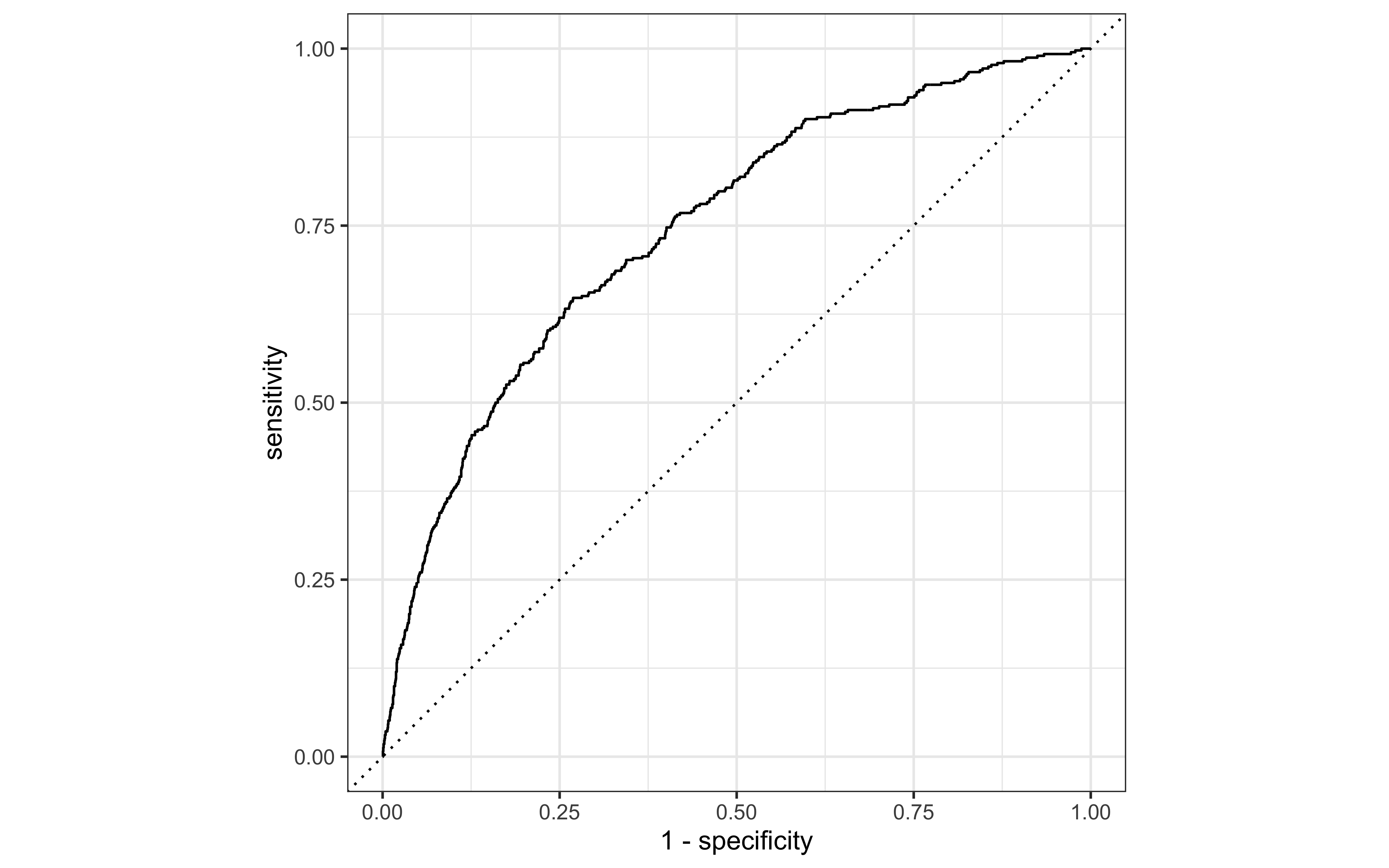

20.1.2 AUC

Similarly, roc_auc() estimates the area under the curve:

flights_pred_lr_mod %>% 
  roc_auc(truth = arr_delay, .pred_late)

## # A tibble: 1 x 3
##   .metric .estimator .estimate
##   <chr>   <chr>          <dbl>
## 1 roc_auc binary         0.746

20.1.3 Accuracy

We use the metrics() function to measure the performance of the model. It will automatically choose metrics appropriate for a given type of model. The function expects a tibble that contains the actual results (truth) and what the model predicted (estimate).

flights_fit_lr_mode %>%
  predict(test_data) %>%
  bind_cols(test_data) %>%
  metrics(truth = arr_delay, 
          estimate = .pred_class)

## # A tibble: 2 x 3
##   .metric  .estimator .estimate
##   <chr>    <chr>          <dbl>
## 1 accuracy binary         0.847
## 2 kap      binary         0.182

20.1.4 Recall

flights_fit_lr_mode %>%
  predict(test_data) %>%
    bind_cols(test_data) %>%
  recall(truth = arr_delay, 
          estimate = .pred_class)

## # A tibble: 1 x 3
##   .metric .estimator .estimate
##   <chr>   <chr>          <dbl>
## 1 recall  binary         0.153

20.1.5 Precision

flights_fit_lr_mode %>%
  predict(test_data) %>%
    bind_cols(test_data) %>%
  precision(truth = arr_delay, 
          estimate = .pred_class)

## # A tibble: 1 x 3
##   .metric   .estimator .estimate
##   <chr>     <chr>          <dbl>
## 1 precision binary         0.541