Linear Regression in Python

Does money make people happier? Version with data splitting.

Data

Import

import pandas as pd

# Load the data from GitHub
LINK = "https://raw.githubusercontent.com/kirenz/datasets/master/oecd_gdp.csv"
df = pd.read_csv(LINK)

df.head()

	Country	GDP per capita	Life satisfaction
0	Russia	9054.914	6.0
1	Turkey	9437.372	5.6
2	Hungary	12239.894	4.9
3	Poland	12495.334	5.8
4	Slovak Republic	15991.736	6.1

df.tail()

	Country	GDP per capita	Life satisfaction
24	Iceland	50854.583	7.5
25	Australia	50961.865	7.3
26	Ireland	51350.744	7.0
27	Denmark	52114.165	7.5
28	United States	55805.204	7.2

df.info()

<class 'pandas.core.frame.DataFrame'>
RangeIndex: 29 entries, 0 to 28
Data columns (total 3 columns):
 #   Column             Non-Null Count  Dtype  
---  ------             --------------  -----  
 0   Country            29 non-null     object 
 1   GDP per capita     29 non-null     float64
 2   Life satisfaction  29 non-null     float64
dtypes: float64(2), object(1)
memory usage: 824.0+ bytes

Correct format

# Change column names 
df.columns = df.columns.str.lower().str.replace(' ', '_')

df.head()

	country	gdp_per_capita	life_satisfaction
0	Russia	9054.914	6.0
1	Turkey	9437.372	5.6
2	Hungary	12239.894	4.9
3	Poland	12495.334	5.8
4	Slovak Republic	15991.736	6.1

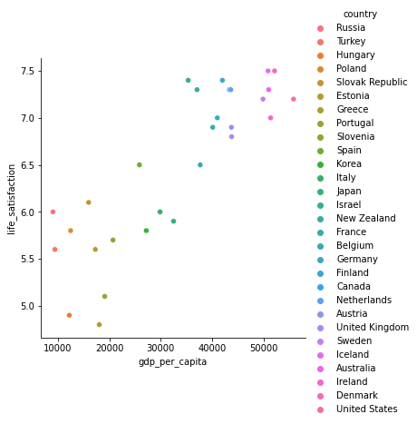
Exploration

%matplotlib inline
import seaborn as sns

# Visualize the data
sns.relplot(x="gdp_per_capita", y='life_satisfaction', hue='country', data=df);

Data split

# Select feature for simple regression
X = df[['gdp_per_capita']]

# Create response
y = df["life_satisfaction"]

from sklearn.model_selection import train_test_split

# Train Test Split
X_train, X_test, y_train, y_test = train_test_split(X, y, test_size=0.2, random_state=42)

Model

Simple linear regression

Training

from sklearn.linear_model import LinearRegression

# Select a linear regression model
reg = LinearRegression()

# Train the model
reg.fit(X_train, y_train)

LinearRegression()

In a Jupyter environment, please rerun this cell to show the HTML representation or trust the notebook.
On GitHub, the HTML representation is unable to render, please try loading this page with nbviewer.org.

# Model coefficients
print('Coefficients: \n', "Intercept:", reg.intercept_, "\n Coefficient:", reg.coef_)

Coefficients: 
 Intercept: 4.867383809184242 
 Coefficient: [4.9184703e-05]

Prediction

# Prediction
y_pred = reg.predict(X_test)

Evaluation

from sklearn.metrics import r2_score

r2_score(y_test, y_pred)

0.7578144582350161

# pretty output
print("Coefficient of determination: %.2f" % r2_score(y_test, y_pred))

Coefficient of determination: 0.76

from sklearn.metrics import mean_squared_error

# Mean squared error
mean_squared_error(y_test, y_pred)

0.09021411430745645

# Root mean squared error
mean_squared_error(y_test, y_pred, squared=False)

0.30035664518611277

Use model

# Create a new GDP value
X_new = pd.DataFrame({"gdp_per_capita": [50000]})

# Make a prediction for new GDP value
reg.predict(X_new)

array([7.32661896])

Save and load model

from pathlib import Path

# show current working directory
Path.cwd()

PosixPath('/home/runner/work/analytics/analytics/docs')

It is possible to save a model in scikit-learn by using joblib’s dump and load:

from joblib import dump, load

# store model in current working directory with Path()
dump(reg, Path('my_linear_model.joblib')) 

['my_linear_model.joblib']

# load model and save it as reg2 
reg2 = load(Path('my_linear_model.joblib')) 

# make a prediction
reg2.predict(X_new)

array([7.32661896])