Chapter 3 Barplot

You should use this method if the data is:

• Categorical

In this chapter you will learn how to do some simple data explorations for categorical variables using barplots.

3.1 One variable

wage_df %>% 
  ggplot(aes(x = maritl)) +
  geom_bar()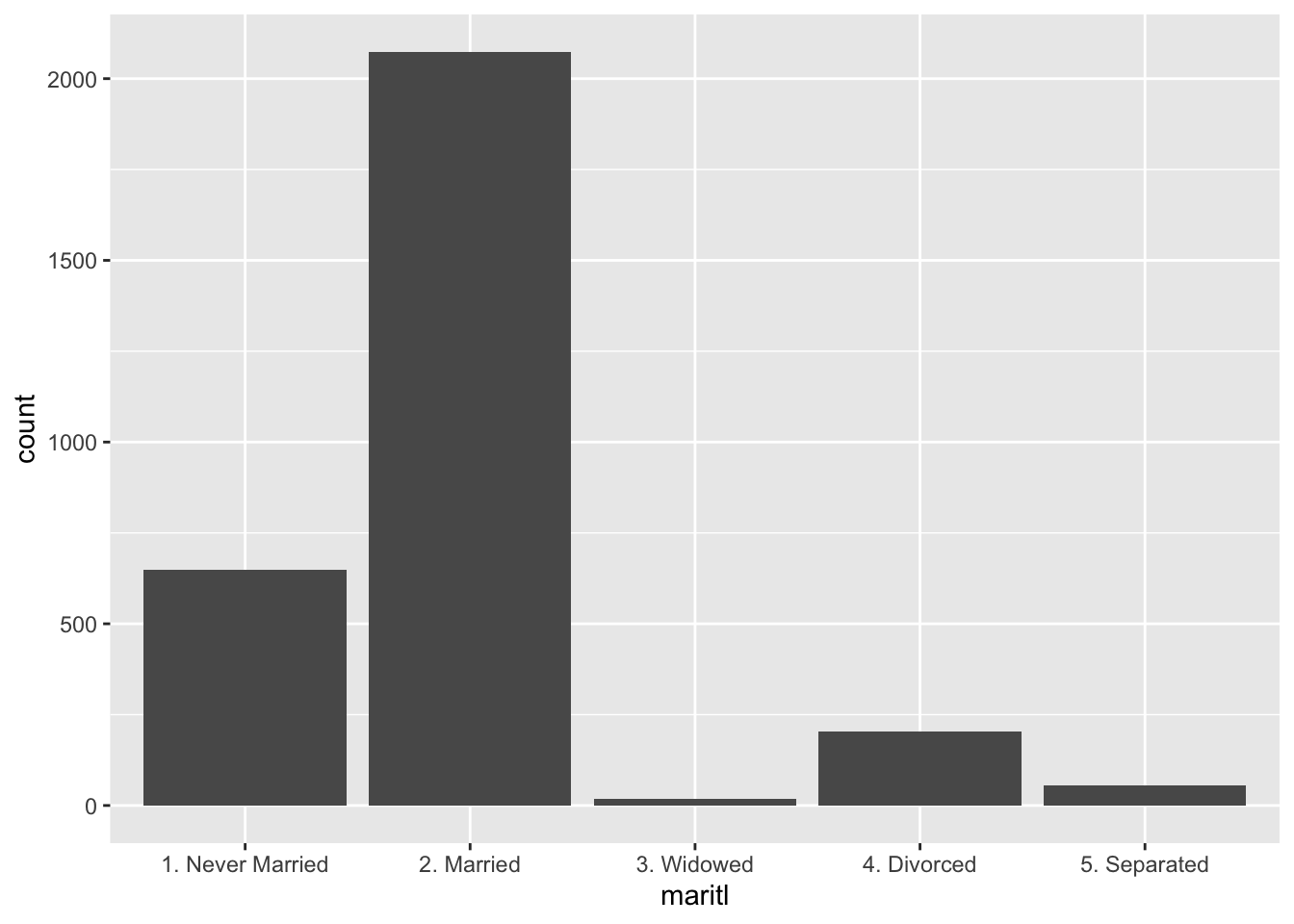

3.2 Two variables

3.2.1 Stacked barplot

Absolute values:

wage_df %>% 
  ggplot(aes(x = maritl, fill = education)) + 
  geom_bar()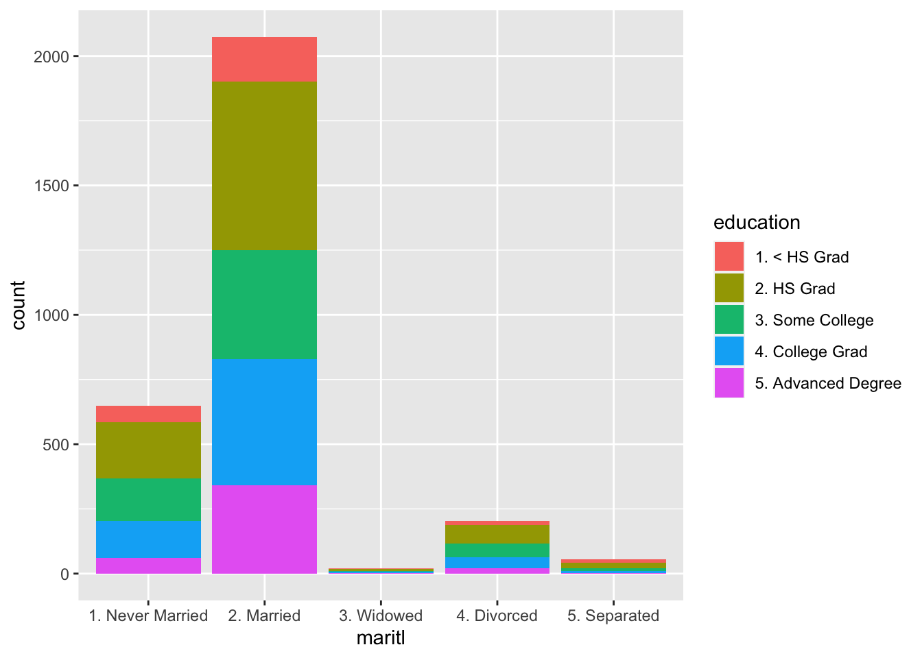

Relative values:

wage_df %>% 
  ggplot(aes(x = maritl, fill = education)) +
  geom_bar(position = "fill") +
  ggtitle("Marital Status", "Overview") +
  xlab(" Marital Status") +
  ylab("Number of People") +
  theme_classic() +
  scale_fill_brewer(palette = "Blues") +
  theme(legend.title = element_blank())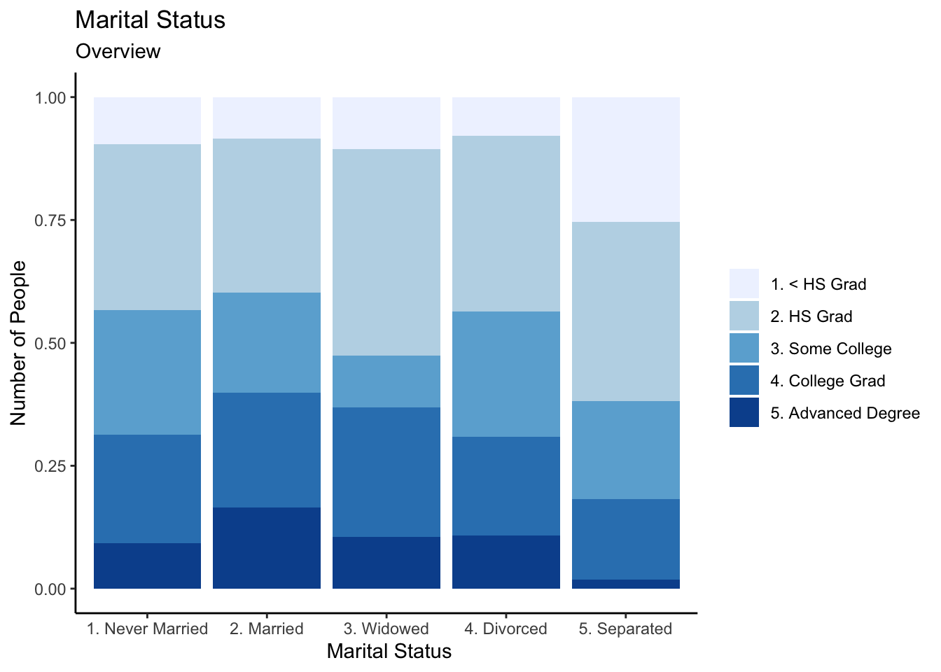

3.2.2 Side-by-side barplot

Basic plot:

wage_df %>% 
  ggplot(aes(x = maritl, fill = education)) +
  geom_bar(position = "dodge")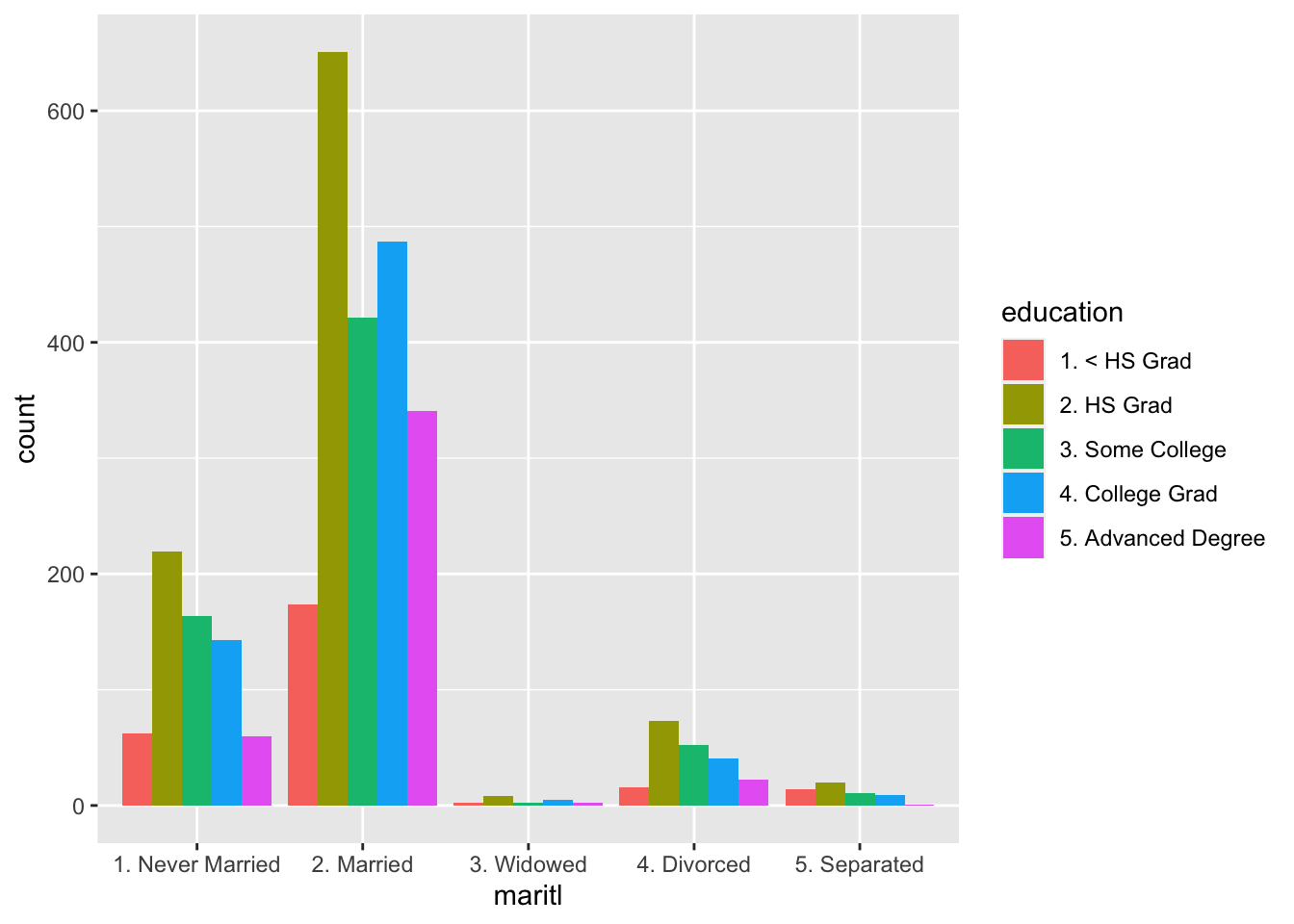 

Plot with some adjustments:

wage_df %>% 
  ggplot(aes(x = maritl, fill = education)) +
  geom_bar(position = "dodge") +
  ggtitle("Marital Status", "Overview") +
  xlab(" Marital Status") +
  ylab("Number of People") +
  theme_classic() +
  scale_fill_brewer(palette = "Blues") +
  theme(legend.title = element_blank())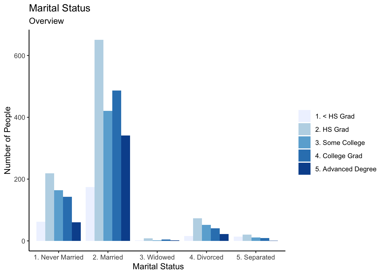

3.2.3 Faceted barplot

Basic plot:

wage_df %>% 
  ggplot(aes(x = maritl)) +
  geom_bar(position = "dodge") +
  facet_wrap(~ education)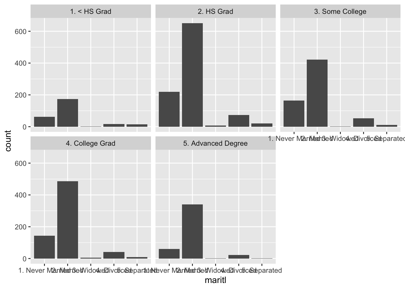

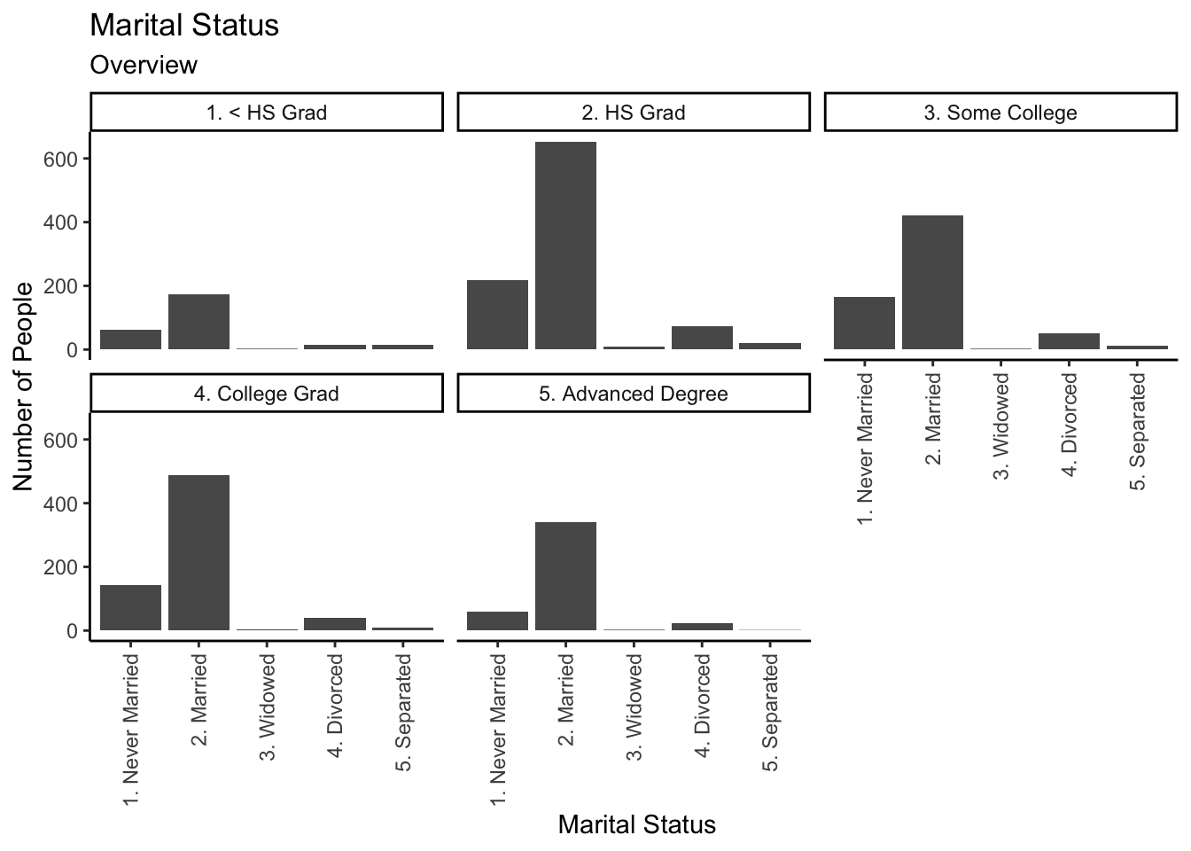
Plot with some adjustments to change our x labels using justifications):

Horizontal and vertical justification have the same parameterisation, either a string (“top,” “middle,” “bottom,” “left,” “center,” “right”) or a number between 0 and 1:"

• top = 1, middle = 0.5, bottom = 0
• left = 0, center = 0.5, right = 1

wage_df %>% 
  ggplot(aes(x = maritl)) +
  geom_bar(position = "dodge") +
  facet_wrap(~ education) + 
  ggtitle("Marital Status", "Overview") +
  xlab(" Marital Status") +
  ylab("Number of People") +
  theme_classic() +
  theme(legend.title = element_blank()) +
  theme(axis.text.x = element_text(angle = 90, 
                                   vjust = 0.5, 
                                   hjust=  1))