Data augmentation#

#@title Licensed under the Apache License, Version 2.0 (the "License");
# you may not use this file except in compliance with the License.
# You may obtain a copy of the License at
#
# https://www.apache.org/licenses/LICENSE-2.0
#
# Unless required by applicable law or agreed to in writing, software
# distributed under the License is distributed on an "AS IS" BASIS,
# WITHOUT WARRANTIES OR CONDITIONS OF ANY KIND, either express or implied.
# See the License for the specific language governing permissions and
# limitations under the License.

Overview#

This tutorial demonstrates data augmentation: a technique to increase the diversity of your training set by applying random (but realistic) transformations, such as image rotation.
You will learn how to apply data augmentation in two ways:
Use the Keras preprocessing layers, such as tf.keras.layers.Resizing, tf.keras.layers.Rescaling, tf.keras.layers.RandomFlip, and tf.keras.layers.RandomRotation.
Use the tf.image methods, such as tf.image.flip_left_right, tf.image.rgb_to_grayscale, tf.image.adjust_brightness, tf.image.central_crop, and tf.image.stateless_random*.

Setup#

import matplotlib.pyplot as plt
import numpy as np
import tensorflow as tf
import tensorflow_datasets as tfds

from tensorflow.keras import layers

Download a dataset#

This tutorial uses the tf_flowers dataset.
For convenience, download the dataset using TensorFlow Datasets.
If you would like to learn about other ways of importing data, check out the load images tutorial.

(train_ds, val_ds, test_ds), metadata = tfds.load(
    'tf_flowers',
    split=['train[:80%]', 'train[80%:90%]', 'train[90%:]'],
    with_info=True,
    as_supervised=True,
)

2022-05-08 19:02:48.919413: W tensorflow/core/platform/cloud/google_auth_provider.cc:184] All attempts to get a Google authentication bearer token failed, returning an empty token. Retrieving token from files failed with "NOT_FOUND: Could not locate the credentials file.". Retrieving token from GCE failed with "FAILED_PRECONDITION: Error executing an HTTP request: libcurl code 6 meaning 'Couldn't resolve host name', error details: Could not resolve host: metadata".

Downloading and preparing dataset 218.21 MiB (download: 218.21 MiB, generated: 221.83 MiB, total: 440.05 MiB) to /Users/jankirenz/tensorflow_datasets/tf_flowers/3.0.1...

Dl Completed...: 100%|██████████| 5/5 [00:06<00:00,  1.23s/ file]

Dataset tf_flowers downloaded and prepared to /Users/jankirenz/tensorflow_datasets/tf_flowers/3.0.1. Subsequent calls will reuse this data.

2022-05-08 19:02:58.394694: I tensorflow/core/platform/cpu_feature_guard.cc:151] This TensorFlow binary is optimized with oneAPI Deep Neural Network Library (oneDNN) to use the following CPU instructions in performance-critical operations:  AVX2 FMA
To enable them in other operations, rebuild TensorFlow with the appropriate compiler flags.

The flowers dataset has five classes.

num_classes = metadata.features['label'].num_classes
print(num_classes)

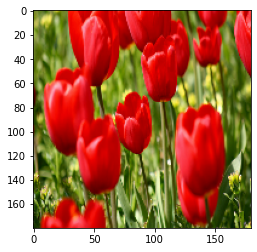
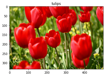
Let’s retrieve an image from the dataset and use it to demonstrate data augmentation.

get_label_name = metadata.features['label'].int2str

image, label = next(iter(train_ds))
_ = plt.imshow(image)
_ = plt.title(get_label_name(label))

2022-05-08 19:03:17.865343: W tensorflow/core/kernels/data/cache_dataset_ops.cc:768] The calling iterator did not fully read the dataset being cached. In order to avoid unexpected truncation of the dataset, the partially cached contents of the dataset  will be discarded. This can happen if you have an input pipeline similar to `dataset.cache().take(k).repeat()`. You should use `dataset.take(k).cache().repeat()` instead.

Use Keras preprocessing layers#

Resizing and rescaling#

You can use the Keras preprocessing layers to resize your images to a consistent shape (with tf.keras.layers.Resizing), and to rescale pixel values (with tf.keras.layers.Rescaling).

IMG_SIZE = 180

resize_and_rescale = tf.keras.Sequential([
  layers.Resizing(IMG_SIZE, IMG_SIZE),
  layers.Rescaling(1./255)
])

Note: The rescaling layer above standardizes pixel values to the [0, 1] range.
If instead you wanted it to be [-1, 1], you would write tf.keras.layers.Rescaling(1./127.5, offset=-1).

You can visualize the result of applying these layers to an image.

result = resize_and_rescale(image)
_ = plt.imshow(result)

Verify that the pixels are in the [0, 1] range:

print("Min and max pixel values:", result.numpy().min(), result.numpy().max())

Min and max pixel values: 0.0 1.0

Data augmentation#

You can use the Keras preprocessing layers for data augmentation as well, such as
- tf.keras.layers.RandomFlip and
- tf.keras.layers.RandomRotation.

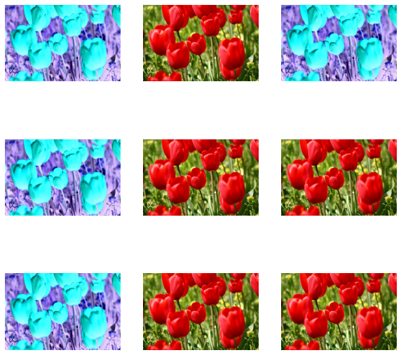
Let’s create a few preprocessing layers and apply them repeatedly to the same image.

data_augmentation = tf.keras.Sequential([
  layers.RandomFlip("horizontal_and_vertical"),
  layers.RandomRotation(0.2),
])

# Add the image to a batch.
image = tf.cast(tf.expand_dims(image, 0), tf.float32)

plt.figure(figsize=(10, 10))
for i in range(9):
  augmented_image = data_augmentation(image)
  ax = plt.subplot(3, 3, i + 1)
  plt.imshow(augmented_image[0])
  plt.axis("off")

WARNING:matplotlib.image:Clipping input data to the valid range for imshow with RGB data ([0..1] for floats or [0..255] for integers).
WARNING:matplotlib.image:Clipping input data to the valid range for imshow with RGB data ([0..1] for floats or [0..255] for integers).
WARNING:matplotlib.image:Clipping input data to the valid range for imshow with RGB data ([0..1] for floats or [0..255] for integers).
WARNING:matplotlib.image:Clipping input data to the valid range for imshow with RGB data ([0..1] for floats or [0..255] for integers).
WARNING:matplotlib.image:Clipping input data to the valid range for imshow with RGB data ([0..1] for floats or [0..255] for integers).
WARNING:matplotlib.image:Clipping input data to the valid range for imshow with RGB data ([0..1] for floats or [0..255] for integers).
WARNING:matplotlib.image:Clipping input data to the valid range for imshow with RGB data ([0..1] for floats or [0..255] for integers).
WARNING:matplotlib.image:Clipping input data to the valid range for imshow with RGB data ([0..1] for floats or [0..255] for integers).
WARNING:matplotlib.image:Clipping input data to the valid range for imshow with RGB data ([0..1] for floats or [0..255] for integers).

There are a variety of preprocessing layers you can use for data augmentation including
- tf.keras.layers.RandomContrast
- tf.keras.layers.RandomCrop
- tf.keras.layers.RandomZoom,

and others.

Two options to use the Keras preprocessing layers#

There are two ways you can use these preprocessing layers, with important trade-offs.

Option 1: Make the preprocessing layers part of your model#

model = tf.keras.Sequential([
  # Add the preprocessing layers you created earlier.
  resize_and_rescale,
  data_augmentation,
  layers.Conv2D(16, 3, padding='same', activation='relu'),
  layers.MaxPooling2D(),
  # Rest of your model.
])

There are two important points to be aware of in this case:

Data augmentation will run on-device, synchronously with the rest of your layers, and benefit from GPU acceleration.
When you export your model using model.save, the preprocessing layers will be saved along with the rest of your model. If you later deploy this model, it will automatically standardize images (according to the configuration of your layers). This can save you from the effort of having to reimplement that logic server-side.

Note: Data augmentation is inactive at test time so input images will only be augmented during calls to Model.fit (not Model.evaluate or Model.predict).

Option 2: Apply the preprocessing layers to your dataset#

aug_ds = train_ds.map(
  lambda x, y: (resize_and_rescale(x, training=True), y))

With this approach, you use Dataset.map to create a dataset that yields batches of augmented images. In this case:

Data augmentation will happen asynchronously on the CPU, and is non-blocking. You can overlap the training of your model on the GPU with data preprocessing, using Dataset.prefetch, shown below.
In this case the preprocessing layers will not be exported with the model when you call Model.save. You will need to attach them to your model before saving it or reimplement them server-side. After training, you can attach the preprocessing layers before export.

You can find an example of the first option in this Image classification tutorial.
Let’s demonstrate the second option here.

Apply the preprocessing layers to the datasets#

Configure the training, validation, and test datasets with the Keras preprocessing layers you created earlier.
You will also configure the datasets for performance, using parallel reads and buffered prefetching to yield batches from disk without I/O become blocking.
Learn more about dataset performance in the Better performance with the tf.data API guide.

Note: Data augmentation should only be applied to the training set.

batch_size = 32
AUTOTUNE = tf.data.AUTOTUNE

def prepare(ds, shuffle=False, augment=False):
  # Resize and rescale all datasets.
  ds = ds.map(lambda x, y: (resize_and_rescale(x), y), 
              num_parallel_calls=AUTOTUNE)

  if shuffle:
    ds = ds.shuffle(1000)

  # Batch all datasets.
  ds = ds.batch(batch_size)

  # Use data augmentation only on the training set.
  if augment:
    ds = ds.map(lambda x, y: (data_augmentation(x, training=True), y), 
                num_parallel_calls=AUTOTUNE)

  # Use buffered prefetching on all datasets.
  return ds.prefetch(buffer_size=AUTOTUNE)

train_ds = prepare(train_ds, shuffle=True, augment=True)
val_ds = prepare(val_ds)
test_ds = prepare(test_ds)

Train a model#

For completeness, you will now train a sequential model using the datasets you have just prepared.
The Sequential model consists of three convolution blocks (tf.keras.layers.Conv2D) with a max pooling layer (tf.keras.layers.MaxPooling2D) in each of them.
There’s a fully-connected layer (tf.keras.layers.Dense) with 128 units on top of it that is activated by a ReLU activation function ('relu').
This model has not been tuned for accuracy (the goal is to show you the mechanics).

model = tf.keras.Sequential([
  
  layers.Conv2D(16, 3, padding='same', activation='relu'),
  layers.MaxPooling2D(),
  
  layers.Conv2D(32, 3, padding='same', activation='relu'),
  layers.MaxPooling2D(),
  
  layers.Conv2D(64, 3, padding='same', activation='relu'),
  layers.MaxPooling2D(),
  
    
  layers.Flatten(),
  layers.Dense(128, activation='relu'),
    
  layers.Dense(num_classes)
])

Choose the tf.keras.optimizers.Adam optimizer and tf.keras.losses.SparseCategoricalCrossentropy loss function.
To view training and validation accuracy for each training epoch, pass the metrics argument to Model.compile.

model.compile(optimizer='adam',
              loss=tf.keras.losses.SparseCategoricalCrossentropy(from_logits=True),
              metrics=['accuracy'])

Train for a few epochs:

epochs=5
history = model.fit(
  train_ds,
  validation_data=val_ds,
  epochs=epochs
)

Epoch 1/5
92/92 [==============================] - 22s 223ms/step - loss: 1.4549 - accuracy: 0.3767 - val_loss: 1.1546 - val_accuracy: 0.5559
Epoch 2/5
92/92 [==============================] - 20s 216ms/step - loss: 1.1224 - accuracy: 0.5433 - val_loss: 1.0648 - val_accuracy: 0.6049
Epoch 3/5
92/92 [==============================] - 20s 216ms/step - loss: 1.0072 - accuracy: 0.5858 - val_loss: 1.0126 - val_accuracy: 0.6158
Epoch 4/5
92/92 [==============================] - 20s 218ms/step - loss: 0.9506 - accuracy: 0.6223 - val_loss: 0.9392 - val_accuracy: 0.6376
Epoch 5/5
92/92 [==============================] - 20s 217ms/step - loss: 0.8954 - accuracy: 0.6468 - val_loss: 1.0059 - val_accuracy: 0.5477

loss, acc = model.evaluate(test_ds)
print("Accuracy", acc)

12/12 [==============================] - 1s 60ms/step - loss: 0.9189 - accuracy: 0.6076
Accuracy 0.6076294183731079

Custom data augmentation#

You can also create custom data augmentation layers.
This section of the tutorial shows two ways of doing so:
First, you will create a tf.keras.layers.Lambda layer. This is a good way to write concise code.
Next, you will write a new layer via subclassing, which gives you more control.

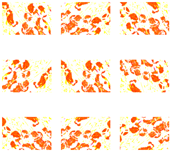
Both layers will randomly invert the colors in an image, according to some probability.

def random_invert_img(x, p=0.5):
  if  tf.random.uniform([]) < p:
    x = (255-x)
  else:
    x
  return x

def random_invert(factor=0.5):
  return layers.Lambda(lambda x: random_invert_img(x, factor))

random_invert = random_invert()

plt.figure(figsize=(10, 10))
for i in range(9):
  augmented_image = random_invert(image)
  ax = plt.subplot(3, 3, i + 1)
  plt.imshow(augmented_image[0].numpy().astype("uint8"))
  plt.axis("off")

Next, implement a custom layer by subclassing:

class RandomInvert(layers.Layer):
  def __init__(self, factor=0.5, **kwargs):
    super().__init__(**kwargs)
    self.factor = factor

  def call(self, x):
    return random_invert_img(x)

_ = plt.imshow(RandomInvert()(image)[0])

WARNING:matplotlib.image:Clipping input data to the valid range for imshow with RGB data ([0..1] for floats or [0..255] for integers).

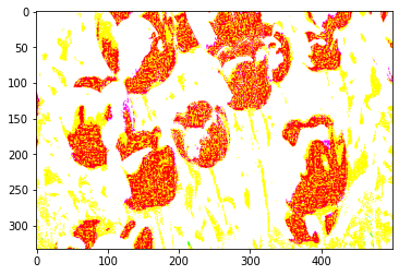
Both of these layers can be used as described in options 1 and 2 above.

Using tf.image#

The above Keras preprocessing utilities are convenient.
But, for finer control, you can write your own data augmentation pipelines or layers using tf.data and tf.image.
You may also want to check out TensorFlow Addons Image: Operations and TensorFlow I/O: Color Space Conversions.

Since the flowers dataset was previously configured with data augmentation, let’s reimport it to start fresh:

(train_ds, val_ds, test_ds), metadata = tfds.load(
    'tf_flowers',
    split=['train[:80%]', 'train[80%:90%]', 'train[90%:]'],
    with_info=True,
    as_supervised=True,
)

Retrieve an image to work with:

image, label = next(iter(train_ds))
_ = plt.imshow(image)
_ = plt.title(get_label_name(label))

2022-05-08 20:14:01.258148: W tensorflow/core/kernels/data/cache_dataset_ops.cc:768] The calling iterator did not fully read the dataset being cached. In order to avoid unexpected truncation of the dataset, the partially cached contents of the dataset  will be discarded. This can happen if you have an input pipeline similar to `dataset.cache().take(k).repeat()`. You should use `dataset.take(k).cache().repeat()` instead.

Let’s use the following function to visualize and compare the original and augmented images side-by-side:

def visualize(original, augmented):
  fig = plt.figure()
  plt.subplot(1,2,1)
  plt.title('Original image')
  plt.imshow(original)

  plt.subplot(1,2,2)
  plt.title('Augmented image')
  plt.imshow(augmented)

Data augmentation#

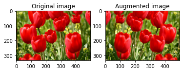
Flip an image#

Flip an image either vertically or horizontally with tf.image.flip_left_right:

flipped = tf.image.flip_left_right(image)
visualize(image, flipped)

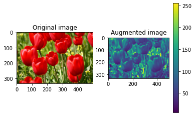
Grayscale an image#

You can grayscale an image with tf.image.rgb_to_grayscale:

grayscaled = tf.image.rgb_to_grayscale(image)
visualize(image, tf.squeeze(grayscaled))
_ = plt.colorbar()

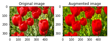
Saturate an image#

Saturate an image with tf.image.adjust_saturation by providing a saturation factor:

saturated = tf.image.adjust_saturation(image, 3)
visualize(image, saturated)

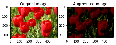
Change image brightness#

Change the brightness of image with tf.image.adjust_brightness by providing a brightness factor:

bright = tf.image.adjust_brightness(image, 0.4)
visualize(image, bright)

Center crop an image#

Crop the image from center up to the image part you desire using tf.image.central_crop:

cropped = tf.image.central_crop(image, central_fraction=0.5)
visualize(image, cropped)

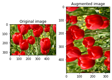
Rotate an image#

Rotate an image by 90 degrees with tf.image.rot90:

rotated = tf.image.rot90(image)
visualize(image, rotated)

Random transformations#

Warning: There are two sets of random image operations: tf.image.random* and tf.image.stateless_random*. Using tf.image.random* operations is strongly discouraged as they use the old RNGs from TF 1.x. Instead, please use the random image operations introduced in this tutorial. For more information, refer to Random number generation.
Applying random transformations to the images can further help generalize and expand the dataset.

The current tf.image API provides eight such random image operations (ops):

These random image ops are purely functional: the output only depends on the input.
This makes them simple to use in high performance, deterministic input pipelines.
They require a seed value be input each step. Given the same seed, they return the same results independent of how many times they are called.

Note: seed is a Tensor of shape (2,) whose values are any integers.

In the following sections, you will:

Go over examples of using random image operations to transform an image.
Demonstrate how to apply random transformations to a training dataset.

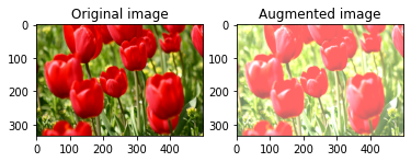
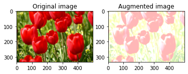
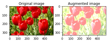
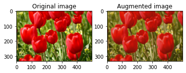
Randomly change image brightness#

Randomly change the brightness of image using tf.image.stateless_random_brightness by providing a brightness factor and seed. The brightness factor is chosen randomly in the range [-max_delta, max_delta) and is associated with the given seed.

for i in range(3):
  seed = (i, 0)  # tuple of size (2,)
  stateless_random_brightness = tf.image.stateless_random_brightness(
      image, max_delta=0.95, seed=seed)
  visualize(image, stateless_random_brightness)

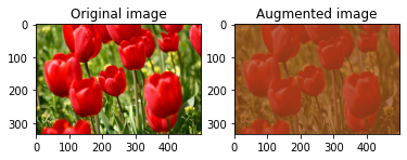
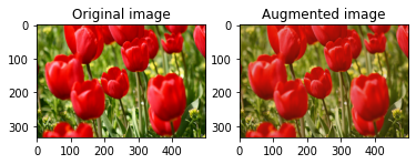
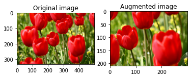
Randomly change image contrast#

-Randomly change the contrast of image using tf.image.stateless_random_contrast by providing a contrast range and seed. The contrast range is chosen randomly in the interval [lower, upper] and is associated with the given seed.

for i in range(3):
  seed = (i, 0)  # tuple of size (2,)
  stateless_random_contrast = tf.image.stateless_random_contrast(
      image, lower=0.1, upper=0.9, seed=seed)
  visualize(image, stateless_random_contrast)

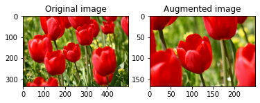
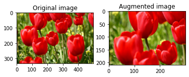
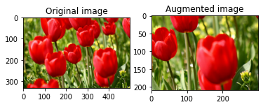
Randomly crop an image#

Randomly crop image using tf.image.stateless_random_crop by providing target size and seed. The portion that gets cropped out of image is at a randomly chosen offset and is associated with the given seed.

for i in range(3):
  seed = (i, 0)  # tuple of size (2,)
  stateless_random_crop = tf.image.stateless_random_crop(
      image, size=[210, 300, 3], seed=seed)
  visualize(image, stateless_random_crop)

Apply augmentation to a dataset#

Let’s first download the image dataset again in case they are modified in the previous sections.

(train_datasets, val_ds, test_ds), metadata = tfds.load(
    'tf_flowers',
    split=['train[:80%]', 'train[80%:90%]', 'train[90%:]'],
    with_info=True,
    as_supervised=True,
)

Next, define a utility function for resizing and rescaling the images. This function will be used in unifying the size and scale of images in the dataset:

def resize_and_rescale(image, label):
  image = tf.cast(image, tf.float32)
  image = tf.image.resize(image, [IMG_SIZE, IMG_SIZE])
  image = (image / 255.0)
  return image, label

Let’s also define the augment function that can apply the random transformations to the images. This function will be used on the dataset in the next step.

def augment(image_label, seed):
  image, label = image_label
  image, label = resize_and_rescale(image, label)
  image = tf.image.resize_with_crop_or_pad(image, IMG_SIZE + 6, IMG_SIZE + 6)
  # Make a new seed.
  new_seed = tf.random.experimental.stateless_split(seed, num=1)[0, :]
  # Random crop back to the original size.
  image = tf.image.stateless_random_crop(
      image, size=[IMG_SIZE, IMG_SIZE, 3], seed=seed)
  # Random brightness.
  image = tf.image.stateless_random_brightness(
      image, max_delta=0.5, seed=new_seed)
  image = tf.clip_by_value(image, 0, 1)
  return image, label

Option 1: Using tf.data.experimental.Counter#

Create a tf.data.experimental.Counter object (let’s call it counter) and Dataset.zip the dataset with (counter, counter). This will ensure that each image in the dataset gets associated with a unique value (of shape (2,)) based on counter which later can get passed into the augment function as the seed value for random transformations.

# Create a `Counter` object and `Dataset.zip` it together with the training set.
counter = tf.data.experimental.Counter()
train_ds = tf.data.Dataset.zip((train_datasets, (counter, counter)))

Map the augment function to the training dataset:

train_ds = (
    train_ds
    .shuffle(1000)
    .map(augment, num_parallel_calls=AUTOTUNE)
    .batch(batch_size)
    .prefetch(AUTOTUNE)
)

val_ds = (
    val_ds
    .map(resize_and_rescale, num_parallel_calls=AUTOTUNE)
    .batch(batch_size)
    .prefetch(AUTOTUNE)
)

test_ds = (
    test_ds
    .map(resize_and_rescale, num_parallel_calls=AUTOTUNE)
    .batch(batch_size)
    .prefetch(AUTOTUNE)
)

Option 2: Using tf.random.Generator#

Create a tf.random.Generator object with an initial seed value. Calling the make_seeds function on the same generator object always returns a new, unique seed value.
Define a wrapper function that: 1) calls the make_seeds function; and 2) passes the newly generated seed value into the augment function for random transformations.

Note: tf.random.Generator objects store RNG state in a tf.Variable, which means it can be saved as a checkpoint or in a SavedModel. For more details, please refer to Random number generation.

# Create a generator.
rng = tf.random.Generator.from_seed(123, alg='philox')

# Create a wrapper function for updating seeds.
def f(x, y):
  seed = rng.make_seeds(2)[0]
  image, label = augment((x, y), seed)
  return image, label

Map the wrapper function f to the training dataset, and the resize_and_rescale function—to the validation and test sets:

train_ds = (
    train_datasets
    .shuffle(1000)
    .map(f, num_parallel_calls=AUTOTUNE)
    .batch(batch_size)
    .prefetch(AUTOTUNE)
)

val_ds = (
    val_ds
    .map(resize_and_rescale, num_parallel_calls=AUTOTUNE)
    .batch(batch_size)
    .prefetch(AUTOTUNE)
)

test_ds = (
    test_ds
    .map(resize_and_rescale, num_parallel_calls=AUTOTUNE)
    .batch(batch_size)
    .prefetch(AUTOTUNE)
)

These datasets can now be used to train a model as shown previously.

Next steps#

This tutorial demonstrated data augmentation using Keras preprocessing layers and tf.image.

To learn how to include preprocessing layers inside your model, refer to the Image classification tutorial.
You may also be interested in learning how preprocessing layers can help you classify text, as shown in the Basic text classification tutorial.
You can learn more about tf.data in this guide, and you can learn how to configure your input pipelines for performance here.

Deep Learning

Data augmentation

Contents

Data augmentation#

Overview#

Setup#

Download a dataset#

Use Keras preprocessing layers#

Resizing and rescaling#

Data augmentation#

Two options to use the Keras preprocessing layers#

Option 1: Make the preprocessing layers part of your model#

Option 2: Apply the preprocessing layers to your dataset#

Apply the preprocessing layers to the datasets#

Train a model#

Custom data augmentation#

Using tf.image#

Data augmentation#

Flip an image#

Grayscale an image#

Saturate an image#

Change image brightness#

Center crop an image#

Rotate an image#

Random transformations#

Randomly change image brightness#

Randomly change image contrast#

Randomly crop an image#

Apply augmentation to a dataset#

Option 1: Using tf.data.experimental.Counter#

Option 2: Using tf.random.Generator#

Next steps#