Image preprocessing and data augmentation#

The following tutorial is based on:

Author: fchollet
Date created: 2020/04/27
Last modified: 2020/04/28
Description: Training an image classifier from scratch on the Kaggle Cats vs Dogs dataset.

Keras provides multiple functions for image processing as well as data augmentation. In this tuorial, we demonstrate how to use some of them.

Image classification#

Image preprocessing#

These layers are for standardizing the inputs of an image model:
- tf.keras.layers.Resizing: resizes a batch of images to a target size.
- tf.keras.layers.Rescaling: rescales and offsets the values of a batch of image (e.g. go from inputs in the [0, 255] range to inputs in the [0, 1] range.
- tf.keras.layers.CenterCrop: returns a center crop of a batch of images.
- Review the Keras image preprocessing documentation to learn more.

Image augmentation#

These layers apply random augmentation transforms to a batch of images (they are only active during training):
- tf.keras.layers.RandomCrop
- tf.keras.layers.RandomFlip
- tf.keras.layers.RandomTranslation
- tf.keras.layers.RandomRotation
- tf.keras.layers.RandomZoom
- tf.keras.layers.RandomHeight
- tf.keras.layers.RandomWidth
- tf.keras.layers.RandomContrast

Review the Keras image data augmentation documentation to learn more.

Introduction#

This example shows how to do image classification from scratch, starting from JPEG image files on disk, without leveraging pre-trained weights or a pre-made Keras Application model.
We demonstrate the workflow on the Kaggle Cats vs Dogs binary classification dataset.
We use the image_dataset_from_directory utility to generate the datasets, and we use Keras image preprocessing layers for image standardization and data augmentation.

Setup#

import tensorflow as tf
from tensorflow import keras
from tensorflow.keras import layers

Load the data: the Cats vs Dogs dataset#

Raw data download#

First, let’s download the 786M ZIP archive of the raw data:

!curl -O https://download.microsoft.com/download/3/E/1/3E1C3F21-ECDB-4869-8368-6DEBA77B919F/kagglecatsanddogs_3367a.zip

  % Total    % Received % Xferd  Average Speed   Time    Time     Time  Current
                                 Dload  Upload   Total   Spent    Left  Speed
100  786M  100  786M    0     0  22.7M      0  0:00:34  0:00:34 --:--:-- 22.2M

!unzip -q kagglecatsanddogs_3367a.zip
!ls

replace MSR-LA - 3467.docx? [y]es, [n]o, [A]ll, [N]one, [r]ename: ^C
MSR-LA - 3467.docx
PetImages
cnn.ipynb
convolutional-nn.ipynb
convolutional.md
data-import-preprocessing.ipynb
deep-learning.md
fashion-mnist-exercises-solution.ipynb
fashion-mnist-exercises.ipynb
fashion-mnist.ipynb
hugging-face.md
image_augmentation.ipynb
image_classification_from_scratch.ipynb
imdb_model
intro.md
jena_climate_2009_2016.csv
jena_climate_2009_2016.csv.zip
jena_conv.keras
jena_dense.keras
jena_lstm.keras
jena_lstm_dropout.keras
jena_stacked_gru_dropout.keras
kagglecatsanddogs_3367a.zip
keras-functional-c.ipynb
keras-functional.ipynb
keras-imdb-c.ipynb
keras-imdb.ipynb
keras-preprocesing.md
keras-sequential-c.ipynb
keras-sequential.ipynb
keras-subclass-c.ipynb
keras-subclass.ipynb
keras-time-tutorial.ipynb
keras-time.ipynb
keras-timeseries_weather_forecasting.ipynb
keras-tuner.ipynb
logs
mnist-cnn-c.ipynb
mnist-cnn.ipynb
mnist-pytorch.ipynb
mnist-tensorflow.ipynb
model-exercises.ipynb
model.png
my_hd_classifier
readme[1].txt
reference.md
regression-structured.md
save_at_1.h5
save_at_2.h5
sentiment_classifier.png
sentiment_classifier_with_shape_info.png
statquest_introduction_to_pytorch
structured_data_classification_from_scratch-c.ipynb
structured_data_classification_functions.ipynb
structured_data_classification_intro.ipynb
structured_data_classification_layers.ipynb
tensorflow.md
tf-example.ipynb
tf-example.slides.html
ticket_classifier.png
ticket_classifier_with_shape_info.png
time_jena_lstm.keras
time_jena_lstm_dropout.keras
time_jena_stacked_gru_dropout.keras
tmp
updated_ticket_classifier.png

Now we have a PetImages folder which contain two subfolders, Cat and Dog. Each subfolder contains image files for each category.

!ls PetImages

Cat Dog

Filter out corrupted images#

When working with lots of real-world image data, corrupted images are a common occurence.
Let’s filter out badly-encoded images that do not feature the string “JFIF” in their header.

import os

num_skipped = 0
for folder_name in ("Cat", "Dog"):
    folder_path = os.path.join("PetImages", folder_name)
    for fname in os.listdir(folder_path):
        fpath = os.path.join(folder_path, fname)
        try:
            fobj = open(fpath, "rb")
            is_jfif = tf.compat.as_bytes("JFIF") in fobj.peek(10)
        finally:
            fobj.close()

        if not is_jfif:
            num_skipped += 1
            # Delete corrupted image
            os.remove(fpath)

print("Deleted %d images" % num_skipped)

Deleted 1590 images

Generate a `Dataset`#

image_size = (180, 180)
batch_size = 32

train_ds = tf.keras.preprocessing.image_dataset_from_directory(
    "PetImages",
    validation_split=0.2,
    subset="training",
    seed=1337,
    image_size=image_size,
    batch_size=batch_size,
)

Found 23410 files belonging to 2 classes.
Using 18728 files for training.

2022-05-08 17:59:50.702092: I tensorflow/core/platform/cpu_feature_guard.cc:151] This TensorFlow binary is optimized with oneAPI Deep Neural Network Library (oneDNN) to use the following CPU instructions in performance-critical operations:  AVX2 FMA
To enable them in other operations, rebuild TensorFlow with the appropriate compiler flags.

val_ds = tf.keras.preprocessing.image_dataset_from_directory(
    "PetImages",
    validation_split=0.2,
    subset="validation",
    seed=1337,
    image_size=image_size,
    batch_size=batch_size,
)

Found 23410 files belonging to 2 classes.
Using 4682 files for validation.

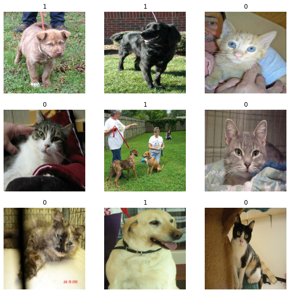
Visualize the data#

Here are the first 9 images in the training dataset.
As you can see, label 1 is “dog” and label 0 is “cat”.

import matplotlib.pyplot as plt

plt.figure(figsize=(10, 10))
for images, labels in train_ds.take(1):
    for i in range(9):
        ax = plt.subplot(3, 3, i + 1)
        plt.imshow(images[i].numpy().astype("uint8"))
        plt.title(int(labels[i]))
        plt.axis("off")

Corrupt JPEG data: 2226 extraneous bytes before marker 0xd9

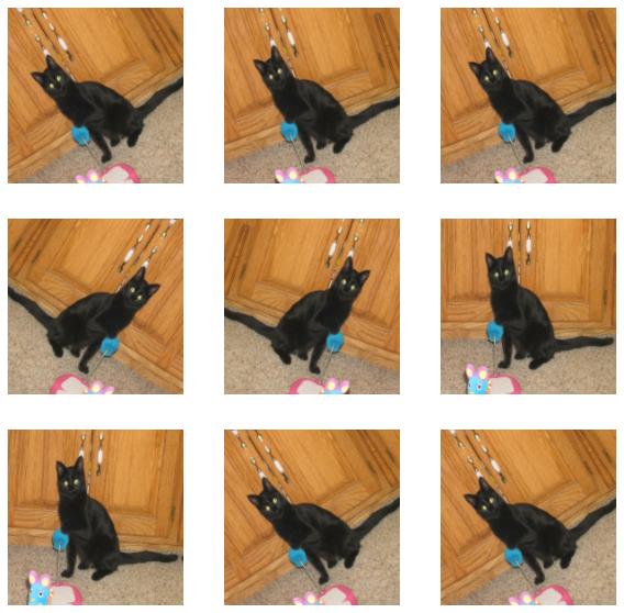
../_images/image_classification_from_scratch_27_1.png

Using image data augmentation#

When you don’t have a large image dataset, it’s a good practice to artificially introduce sample diversity by applying random yet realistic transformations to the training images, such as random horizontal flipping or small random rotations.
This helps expose the model to different aspects of the training data while slowing down overfitting.

data_augmentation = keras.Sequential(
    [
        layers.RandomFlip("horizontal"),
        layers.RandomRotation(0.1),
    ]
)

Let’s visualize what the augmented samples look like, by applying data_augmentation repeatedly to the first image in the dataset:

plt.figure(figsize=(10, 10))
for images, _ in train_ds.take(1):
    for i in range(9):
        augmented_images = data_augmentation(images)
        ax = plt.subplot(3, 3, i + 1)
        plt.imshow(augmented_images[0].numpy().astype("uint8"))
        plt.axis("off")

Corrupt JPEG data: 2226 extraneous bytes before marker 0xd9

../_images/image_classification_from_scratch_32_1.png

Standardizing the data#

Our image are already in a standard size (180x180), as they are being yielded as contiguous float32 batches by our dataset.
However, their RGB channel values are in the [0, 255] range.
This is not ideal for a neural network; in general you should seek to make your input values small.
Here, we will standardize values to be in the [0, 1] by using a Rescaling layer at the start of our model.

Two options to preprocess the data#

There are two ways you could be using the data_augmentation preprocessor:

Option 1: Make it part of the model, like this:

inputs = keras.Input(shape=input_shape)
x = data_augmentation(inputs)
x = layers.Rescaling(1./255)(x)
...  # Rest of the model

With this option, your data augmentation will happen on device, synchronously with the rest of the model execution, meaning that it will benefit from GPU acceleration.
Note that data augmentation is inactive at test time, so the input samples will only be augmented during fit(), not when calling evaluate() or predict().
If you’re training on GPU, this is the better option.

Option 2: apply it to the dataset, so as to obtain a dataset that yields batches of augmented images, like this:

augmented_train_ds = train_ds.map(
  lambda x, y: (data_augmentation(x, training=True), y))

With this option, your data augmentation will happen on CPU, asynchronously, and will be buffered before going into the model.
If you’re training on CPU, this is the better option, since it makes data augmentation asynchronous and non-blocking.

In our case, we’ll go with the first option.

Configure the dataset for performance#

Let’s make sure to use buffered prefetching so we can yield data from disk without having I/O becoming blocking:

train_ds = train_ds.prefetch(buffer_size=32)
val_ds = val_ds.prefetch(buffer_size=32)

Build a model#

Best practice advice#

Convnet architecture principles (Chollet, 2021):

Your model should be organized into repeated blocks of layers, usually made of
- multiple convolution layers (usually Conv2d) and a
- max pooling layer (usually MaxPooling2D).

The number of filters in your layers should increase (usually we double it) as the size of the spatial feature maps decreases.

Deep and narrow is better than broad and shallow.

Introducing residual connections around blocks of layers helps you train deeper networks.

It can be beneficial to introduce batch normalization layers after your convolution layers.

It can be beneficial to replace Conv2D layers with SeparableConv2D layers, which are more parameter-efficient.

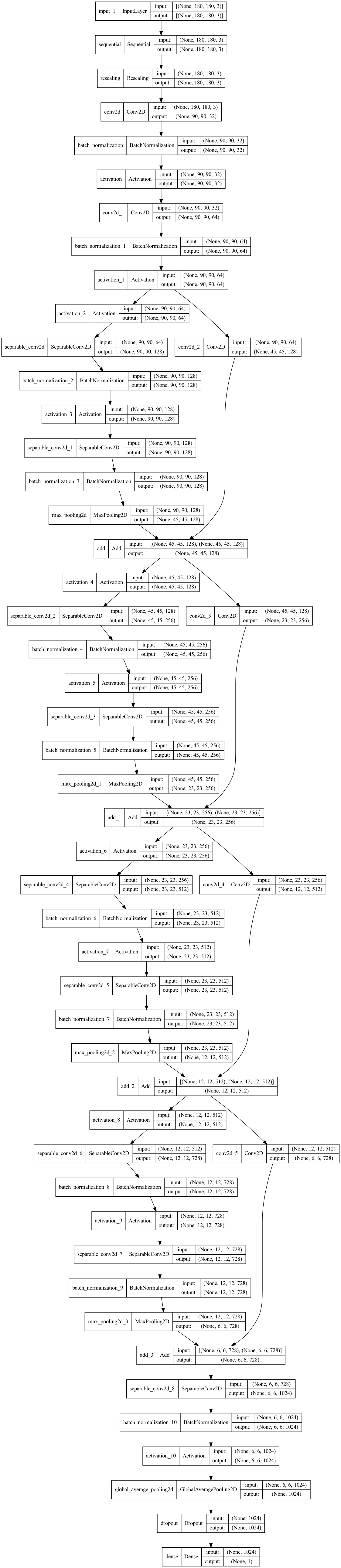
Model#

Next, we’ll build a small version of the Xception network.

Note that:

We start the model with the data_augmentation preprocessor, followed by a Rescaling layer.
first layer in our model is a regular Conv2D layer. We’ll start using SeparableConv2D afterwards

Since the assumption that underlies separable convolution, “feature channels are largely independent,” does not hold for RGB images! Red, green, and blue color channels are actually highly correlated in natural images.

We apply a series of convolutional blocks with increasing feature depth (using a foor loop)

We use GlobalAveragePooling2D -which is similar to flatten the layer- right before the classification outout layer

We include a Dropout layer before the final classification layer.

def make_model(input_shape, num_classes):
 
    inputs = keras.Input(shape=input_shape)
  
    # Image augmentation block
    x = data_augmentation(inputs)

    # Image rescaling
    x = layers.Rescaling(1.0 / 255)(x)

    # Entry block
    
    x = layers.Conv2D(32, 3, strides=2, padding="same")(x)
    x = layers.BatchNormalization()(x)
    x = layers.Activation("relu")(x)

    x = layers.Conv2D(64, 3, padding="same")(x)
    x = layers.BatchNormalization()(x)
    x = layers.Activation("relu")(x)

    previous_block_activation = x  # Set aside residual
    
    # Series of convolutional blocks with SeparableConv2D

    for size in [128, 256, 512, 728]:
        x = layers.Activation("relu")(x)
        x = layers.SeparableConv2D(size, 3, padding="same")(x)
        x = layers.BatchNormalization()(x)

        x = layers.Activation("relu")(x)
        x = layers.SeparableConv2D(size, 3, padding="same")(x)
        x = layers.BatchNormalization()(x)

        x = layers.MaxPooling2D(3, strides=2, padding="same")(x)

        # Project residual
        residual = layers.Conv2D(size, 1, strides=2, padding="same")(
            previous_block_activation
        )
        x = layers.add([x, residual])  # Add back residual
        previous_block_activation = x  # Set aside next residual

             
    x = layers.SeparableConv2D(1024, 3, padding="same")(x)
    x = layers.BatchNormalization()(x)
    x = layers.Activation("relu")(x)

    
    x = layers.GlobalAveragePooling2D()(x)
    if num_classes == 2:
        activation = "sigmoid"
        units = 1
    else:
        activation = "softmax"
        units = num_classes

    x = layers.Dropout(0.5)(x)
    outputs = layers.Dense(units, activation=activation)(x)
    return keras.Model(inputs, outputs)

model = make_model(input_shape=image_size + (3,), num_classes=2)

keras.utils.plot_model(model, show_shapes=True)

../_images/image_classification_from_scratch_63_0.png

We haven’t particularly tried to optimize the architecture; if you want to do a systematic search for the best model configuration, consider using KerasTuner.

Train the model#

epochs = 2 # we only use 2 epochs - you should go with 50

callbacks = [
    keras.callbacks.ModelCheckpoint("save_at_{epoch}.h5"),
]
model.compile(
    optimizer=keras.optimizers.Adam(1e-3),
    loss="binary_crossentropy",
    metrics=["accuracy"],
)
model.fit(
    train_ds, epochs=epochs, callbacks=callbacks, validation_data=val_ds,
)

Epoch 1/2

Corrupt JPEG data: 2226 extraneous bytes before marker 0xd9

293/586 [==============>...............] - ETA: 8:30 - loss: 0.6602 - accuracy: 0.6307

Corrupt JPEG data: 228 extraneous bytes before marker 0xd9

324/586 [===============>..............] - ETA: 7:34 - loss: 0.6528 - accuracy: 0.6353

Warning: unknown JFIF revision number 0.00

402/586 [===================>..........] - ETA: 5:19 - loss: 0.6357 - accuracy: 0.6521

Corrupt JPEG data: 128 extraneous bytes before marker 0xd9

411/586 [====================>.........] - ETA: 5:04 - loss: 0.6341 - accuracy: 0.6531

Corrupt JPEG data: 65 extraneous bytes before marker 0xd9

423/586 [====================>.........] - ETA: 4:43 - loss: 0.6311 - accuracy: 0.6545

Corrupt JPEG data: 396 extraneous bytes before marker 0xd9

430/586 [=====================>........] - ETA: 4:31 - loss: 0.6286 - accuracy: 0.6563

Corrupt JPEG data: 239 extraneous bytes before marker 0xd9

586/586 [==============================] - ETA: 0s - loss: 0.6013 - accuracy: 0.6801

Corrupt JPEG data: 252 extraneous bytes before marker 0xd9
Corrupt JPEG data: 1153 extraneous bytes before marker 0xd9
Corrupt JPEG data: 162 extraneous bytes before marker 0xd9
Corrupt JPEG data: 214 extraneous bytes before marker 0xd9
Corrupt JPEG data: 99 extraneous bytes before marker 0xd9
Corrupt JPEG data: 1403 extraneous bytes before marker 0xd9
/Users/jankirenz/opt/anaconda3/envs/tf/lib/python3.8/site-packages/keras/engine/functional.py:1410: CustomMaskWarning: Custom mask layers require a config and must override get_config. When loading, the custom mask layer must be passed to the custom_objects argument.
  layer_config = serialize_layer_fn(layer)

586/586 [==============================] - 1073s 2s/step - loss: 0.6013 - accuracy: 0.6801 - val_loss: 0.6951 - val_accuracy: 0.6371
Epoch 2/2

Corrupt JPEG data: 2226 extraneous bytes before marker 0xd9

293/586 [==============>...............] - ETA: 8:31 - loss: 0.4708 - accuracy: 0.7811

Corrupt JPEG data: 228 extraneous bytes before marker 0xd9

324/586 [===============>..............] - ETA: 7:37 - loss: 0.4665 - accuracy: 0.7817

Warning: unknown JFIF revision number 0.00

402/586 [===================>..........] - ETA: 5:22 - loss: 0.4626 - accuracy: 0.7848

Corrupt JPEG data: 128 extraneous bytes before marker 0xd9

411/586 [====================>.........] - ETA: 5:06 - loss: 0.4628 - accuracy: 0.7845

Corrupt JPEG data: 65 extraneous bytes before marker 0xd9

423/586 [====================>.........] - ETA: 4:45 - loss: 0.4601 - accuracy: 0.7863

Corrupt JPEG data: 396 extraneous bytes before marker 0xd9

430/586 [=====================>........] - ETA: 4:33 - loss: 0.4588 - accuracy: 0.7873

Corrupt JPEG data: 239 extraneous bytes before marker 0xd9

586/586 [==============================] - ETA: 0s - loss: 0.4448 - accuracy: 0.7942

Corrupt JPEG data: 252 extraneous bytes before marker 0xd9
Corrupt JPEG data: 1153 extraneous bytes before marker 0xd9
Corrupt JPEG data: 162 extraneous bytes before marker 0xd9
Corrupt JPEG data: 214 extraneous bytes before marker 0xd9
Corrupt JPEG data: 99 extraneous bytes before marker 0xd9
Corrupt JPEG data: 1403 extraneous bytes before marker 0xd9

586/586 [==============================] - 1090s 2s/step - loss: 0.4448 - accuracy: 0.7942 - val_loss: 0.3790 - val_accuracy: 0.8321

<keras.callbacks.History at 0x7fa9a1ad1eb0>

We get to ~83% validation accuracy after training for just 2 epochs on the full dataset.
After 50 epochs, it should be around 96%

Run inference on new data#

Note that data augmentation and dropout are inactive at inference time.

img = keras.preprocessing.image.load_img(
    "PetImages/Cat/6779.jpg", target_size=image_size
)

img_array = keras.preprocessing.image.img_to_array(img)

img_array = tf.expand_dims(img_array, 0)  # Create batch axis

predictions = model.predict(img_array)

score = predictions[0]

print(
    "This image is %.2f percent cat and %.2f percent dog."
    % (100 * (1 - score), 100 * score)
)

This image is 91.48 percent cat and 8.52 percent dog.

Deep Learning

Image preprocessing and data augmentation

Contents

Image preprocessing and data augmentation#

Image classification#

Image preprocessing#

Image augmentation#

Introduction#

Setup#

Load the data: the Cats vs Dogs dataset#

Raw data download#

Filter out corrupted images#

Generate a `Dataset`#

Visualize the data#

Using image data augmentation#

Standardizing the data#

Two options to preprocess the data#

Configure the dataset for performance#

Build a model#

Best practice advice#

Model#

Train the model#

Run inference on new data#

Deep Learning

Image preprocessing and data augmentation

Contents

Image preprocessing and data augmentation#

Image classification#

Image preprocessing#

Image augmentation#

Introduction#

Setup#

Load the data: the Cats vs Dogs dataset#

Raw data download#

Filter out corrupted images#

Generate a Dataset#

Visualize the data#

Using image data augmentation#

Standardizing the data#

Two options to preprocess the data#

Configure the dataset for performance#

Build a model#

Best practice advice#

Model#

Train the model#

Run inference on new data#

Generate a `Dataset`#