Classification I#

This tutorial is mainly based on the Keras tutorial “Structured data classification from scratch” by François Chollet.

This example demonstrates how to do structured binary classification with Keras, starting from a raw CSV file.
Our data includes both numerical and categorical features.
We will use Keras preprocessing layers to normalize the numerical features and vectorize the categorical ones.

Note

Note that this example should be run with TensorFlow 2.5 or higher.

Setup#

import pandas as pd

import tensorflow as tf
from tensorflow.keras import layers

tf.__version__

'2.7.1'

Data#

Our dataset is provided by the Cleveland Clinic Foundation for Heart Disease.
It’s a CSV file with 303 rows. Each row contains information about a patient (asample), and each column describes an attribute of the patient (a feature).
We use the features to predict whether a patient has a heart disease (binary classification).

Here’s the description of each feature:

Column	Description	Feature Type
Age	Age in years	Numerical
Sex	(1 = male; 0 = female)	Categorical
CP	Chest pain type (0, 1, 2, 3, 4)	Categorical
Trestbpd	Resting blood pressure (in mm Hg on admission)	Numerical
Chol	Serum cholesterol in mg/dl	Numerical
FBS	fasting blood sugar in 120 mg/dl (1 = true; 0 = false)	Categorical
RestECG	Resting electrocardiogram results (0, 1, 2)	Categorical
Thalach	Maximum heart rate achieved	Numerical
Exang	Exercise induced angina (1 = yes; 0 = no)	Categorical
Oldpeak	ST depression induced by exercise relative to rest	Numerical
Slope	Slope of the peak exercise ST segment	Numerical
CA	Number of major vessels (0-3) colored by fluoroscopy	Both numerical & categorical
Thal	normal; fixed defect; reversible defect	Categorical (string)
Target	Diagnosis of heart disease (1 = true; 0 = false)	Target

The following feature are continuous numerical features:

age
trestbps
chol
thalach
oldpeak
slope

The following features are categorical features encoded as integers:

sex
cp
fbs
restecg
exang
ca

The following feature is a categorical features encoded as string:

thal

Data import#

Let’s download the data and load it into a Pandas dataframe:

file_url = "http://storage.googleapis.com/download.tensorflow.org/data/heart.csv"
df = pd.read_csv(file_url)

Here’s a preview of a few samples:

df.head()

	age	sex	cp	trestbps	chol	fbs	restecg	thalach	exang	oldpeak	slope	ca	thal	target
0	63	1	1	145	233	1	2	150	0	2.3	3	0	fixed	0
1	67	1	4	160	286	0	2	108	1	1.5	2	3	normal	1
2	67	1	4	120	229	0	2	129	1	2.6	2	2	reversible	0
3	37	1	3	130	250	0	0	187	0	3.5	3	0	normal	0
4	41	0	2	130	204	0	2	172	0	1.4	1	0	normal	0

df.info()

<class 'pandas.core.frame.DataFrame'>
RangeIndex: 303 entries, 0 to 302
Data columns (total 14 columns):
 #   Column    Non-Null Count  Dtype  
---  ------    --------------  -----  
 0   age       303 non-null    int64  
 1   sex       303 non-null    int64  
 2   cp        303 non-null    int64  
 3   trestbps  303 non-null    int64  
 4   chol      303 non-null    int64  
 5   fbs       303 non-null    int64  
 6   restecg   303 non-null    int64  
 7   thalach   303 non-null    int64  
 8   exang     303 non-null    int64  
 9   oldpeak   303 non-null    float64
 10  slope     303 non-null    int64  
 11  ca        303 non-null    int64  
 12  thal      303 non-null    object 
 13  target    303 non-null    int64  
dtypes: float64(1), int64(12), object(1)
memory usage: 33.3+ KB

The dataset includes 303 samples with 14 columns per sample (13 features, plus the target label).
The last column, “target”, indicates whether the patient has a heart disease (1) or not (0).

Data splitting#

Let’s split the data into a training and validation set:

df_val = df.sample(frac=0.2, random_state=1337)

df_train = df.drop(df_val.index)

print(
    "Using %d samples for training and %d for validation"
    % (len(df_train), len(df_val))
)

Using 242 samples for training and 61 for validation

Transform to Tensors#

The tf.data.Dataset API supports writing descriptive and efficient input pipelines.
Dataset usage follows a common pattern:
- Create a source dataset from your input data.
- Apply dataset transformations to preprocess the data.
- Iterate over the dataset and process the elements.

Examples#

First, a simple example of how to transform an array into tensors

example_dataset = tf.data.Dataset.from_tensor_slices([1, 2, 3])

# Print tensor
for element in example_dataset:
  print(element)

tf.Tensor(1, shape=(), dtype=int32)
tf.Tensor(2, shape=(), dtype=int32)
tf.Tensor(3, shape=(), dtype=int32)

Example with a dictionary

example_dataset = tf.data.Dataset.from_tensor_slices({"a":[1, 2], "b":[10, 11]} )

# Print tensor
for element in example_dataset:
  print(element)

{'a': <tf.Tensor: shape=(), dtype=int32, numpy=1>, 'b': <tf.Tensor: shape=(), dtype=int32, numpy=10>}
{'a': <tf.Tensor: shape=(), dtype=int32, numpy=2>, 'b': <tf.Tensor: shape=(), dtype=int32, numpy=11>}

How to use dictionary in combination with pandas dataframe

# We only use 1 patient
example_dataset = tf.data.Dataset.from_tensor_slices(dict(df[0:1]))

for element in example_dataset:
  print(element)

{'age': <tf.Tensor: shape=(), dtype=int64, numpy=63>, 'sex': <tf.Tensor: shape=(), dtype=int64, numpy=1>, 'cp': <tf.Tensor: shape=(), dtype=int64, numpy=1>, 'trestbps': <tf.Tensor: shape=(), dtype=int64, numpy=145>, 'chol': <tf.Tensor: shape=(), dtype=int64, numpy=233>, 'fbs': <tf.Tensor: shape=(), dtype=int64, numpy=1>, 'restecg': <tf.Tensor: shape=(), dtype=int64, numpy=2>, 'thalach': <tf.Tensor: shape=(), dtype=int64, numpy=150>, 'exang': <tf.Tensor: shape=(), dtype=int64, numpy=0>, 'oldpeak': <tf.Tensor: shape=(), dtype=float64, numpy=2.3>, 'slope': <tf.Tensor: shape=(), dtype=int64, numpy=3>, 'ca': <tf.Tensor: shape=(), dtype=int64, numpy=0>, 'thal': <tf.Tensor: shape=(), dtype=string, numpy=b'fixed'>, 'target': <tf.Tensor: shape=(), dtype=int64, numpy=0>}

Transformation function#

Let’s generate tf.data.Dataset objects for our training and validation dataframes.
The following utility function converts each training and validation set into a tf.data.Dataset, then shuffles and batches the data.

# Define a function to create our tensors
def dataframe_to_dataset(dataframe, shuffle=True, batch_size=32):
    
    # Make a copy of our dataframe
    df = dataframe.copy()
    # Obtain label and drop target from dataframe
    labels = df.pop("target")

    # Transform data to tensor dataset
    ds = tf.data.Dataset.from_tensor_slices((dict(df), labels))
    
    # Shuffle data
    if shuffle:
        ds = ds.shuffle(buffer_size=len(dataframe))
    
    # Create batches 
    ds = ds.batch(batch_size)
    # Prefetch data for computational efficiency
    df = ds.prefetch(batch_size)

    return ds

Next, we test our function
We use a small batch size to keep the output readable

batch_size = 5

ds_train_test = dataframe_to_dataset(df_train, shuffle=True, batch_size=batch_size)

Let’s take a look at the data:

[(train_features, label_batch)] = ds_train_test.take(1)

print('Every feature:', list(train_features.keys()))
print('A batch of ages:', train_features['age'])
print('A batch of targets:', label_batch )

Every feature: ['age', 'sex', 'cp', 'trestbps', 'chol', 'fbs', 'restecg', 'thalach', 'exang', 'oldpeak', 'slope', 'ca', 'thal']
A batch of ages: tf.Tensor([54 63 65 54 35], shape=(5,), dtype=int64)
A batch of targets: tf.Tensor([0 0 1 1 0], shape=(5,), dtype=int64)

As the output demonstrates, the training set returns a dictionary of column names (from the DataFrame) that map to column values from rows.

Use transformation function#

Let’s now create a input pipeline with a batch size of 32:

# Use function
batch_size = 32

ds_train = dataframe_to_dataset(df_train, shuffle=True, batch_size=batch_size)
ds_val = dataframe_to_dataset(df_val, shuffle=True, batch_size=batch_size)

Feature preprocessing#

Next, we perform feature preprocessing with Keras layers.

Categorical features#

Remember that the following features are categorical features encoded as integers:
- sex
- cp
- fbs
- restecg
- exang
- ca

First, we need to decide how to represent the categorical data

Option 1: One-hot encoding

Example: a color feature gets a 1 in a specific index for different colors (‘red’ = [0, 0, 1, 0, 0])

Option 2: Embed the feature

Example: each color maps to a unique trainable vector (‘red’ = [0.1, 0.2, 0.5, -0.2]

Note

As a rule of thumb: Larger category spaces might do better with an embedding; smaller spaces can use one-hot encoding

We will encode these features using one-hot encoding. We have two options here:
- Use CategoryEncoding(), which requires knowing the range of input values and will error on input outside the range.
- Use IntegerLookup() which will build a lookup table for inputs and reserve an output index for unkown input values.

For this example, we want a simple solution that will handle out of range inputs at inference, so we will use IntegerLookup().

We also have a categorical feature encoded as a string: thal.
We will create an index of all possible features and encode output using the StringLookup() layer.

Numeric features#

The following feature are numerical features:
- age
- trestbps
- chol
- thalach
- oldpeak
- slope

For each of these features, we will use a Normalization() layer to make sure the mean of each feature is 0 and its standard deviation is 1.

Numerical preprocessing functions#

Next, we define a utility function to do the feature preprocessing operations
We create the function encode_numerical_feature to apply featurewise normalization to numerical features.

# Define numerical preprocessing function
def encode_numerical_feature(feature, name, dataset):

    # Create a Normalization layer for our feature
    normalizer = layers.Normalization()

    # Prepare a Dataset that only yields our feature
    feature_ds = dataset.map(lambda x, y: x[name])
    feature_ds = feature_ds.map(lambda x: tf.expand_dims(x, -1))

    # Learn the statistics of the data
    normalizer.adapt(feature_ds)

    # Normalize the input feature
    encoded_feature = normalizer(feature)
    
    return encoded_feature

We use tf.expand_dims(input, axis, name=None) to return a tensor with a length 1 axis inserted at index axis -1.
A negative axis counts from the end so axis=-1 adds an inner most dimension.

Categorical preprocessing functions#

In our function, we handle two types of categorical data:
- if the data type is a string: turn string inputs into integer indices, then one-hot encode these integer indices.
- if the data type is an integer: one-hot encode integer categorical features.

During adapt(), the layer will analyze a data set, determine the frequency of individual strings tokens, and create a vocabulary from them.

# Define categorical preprocessing function
def encode_categorical_feature(feature, name, dataset, is_string):

    # Use StringLookup for datatype string; otherwise use IntegerLookup
    lookup_class = layers.StringLookup if is_string else layers.IntegerLookup
    
    # Create a lookup layer which will turn strings into integer indices
    lookup = lookup_class(output_mode="binary")

    # Prepare a Dataset that only yields our feature
    feature_ds = dataset.map(lambda x, y: x[name])
    feature_ds = feature_ds.map(lambda x: tf.expand_dims(x, -1))

    # Learn the set of possible string values and assign them a fixed integer index
    lookup.adapt(feature_ds)

    # Turn the string input into integer indices
    encoded_feature = lookup(feature)
    
    return encoded_feature

With this done, we can create our preprocessing steps.

Data preprocessing#

In this notebook, we don’t use functions to perform our data preprocessing
Instead, we take care of every feature indivdually

First, we define keras.Input for every feature:

# Categorical features encoded as integers
sex = tf.keras.Input(shape=(1,), name="sex", dtype="int64")
cp = tf.keras.Input(shape=(1,), name="cp", dtype="int64")
fbs = tf.keras.Input(shape=(1,), name="fbs", dtype="int64")
restecg = tf.keras.Input(shape=(1,), name="restecg", dtype="int64")
exang = tf.keras.Input(shape=(1,), name="exang", dtype="int64")
ca = tf.keras.Input(shape=(1,), name="ca", dtype="int64")

# Categorical feature encoded as string
thal = tf.keras.Input(shape=(1,), name="thal", dtype="string")

# Numerical features
age = tf.keras.Input(shape=(1,), name="age")
trestbps = tf.keras.Input(shape=(1,), name="trestbps")
chol = tf.keras.Input(shape=(1,), name="chol")
thalach = tf.keras.Input(shape=(1,), name="thalach")
oldpeak = tf.keras.Input(shape=(1,), name="oldpeak")
slope = tf.keras.Input(shape=(1,), name="slope")

Perform preprocessing with our functions:

# Integer categorical features
sex_encoded = encode_categorical_feature(sex, "sex", ds_train, False)
cp_encoded = encode_categorical_feature(cp, "cp", ds_train, False)
fbs_encoded = encode_categorical_feature(fbs, "fbs", ds_train, False)
restecg_encoded = encode_categorical_feature(restecg, "restecg", ds_train, False)
exang_encoded = encode_categorical_feature(exang, "exang", ds_train, False)
ca_encoded = encode_categorical_feature(ca, "ca", ds_train, False)

# String categorical features
thal_encoded = encode_categorical_feature(thal, "thal", ds_train, True)

# Numerical features
age_encoded = encode_numerical_feature(age, "age", ds_train)
trestbps_encoded = encode_numerical_feature(trestbps, "trestbps", ds_train)
chol_encoded = encode_numerical_feature(chol, "chol", ds_train)
thalach_encoded = encode_numerical_feature(thalach, "thalach", ds_train)
oldpeak_encoded = encode_numerical_feature(oldpeak, "oldpeak", ds_train)
slope_encoded = encode_numerical_feature(slope, "slope", ds_train)

Merge the list of encoded feature inputs (encoded_features) into one vector via concatenation with layers.concatenate:

all_features = layers.concatenate(
    [
        sex_encoded,
        cp_encoded,
        fbs_encoded,
        restecg_encoded,
        exang_encoded,
        ca_encoded,
        thal_encoded,
        age_encoded,
        trestbps_encoded,
        chol_encoded,
        thalach_encoded,
        oldpeak_encoded,
        slope_encoded,
    ]
)

Make a list of all keras.Input feature names

all_inputs = [
    sex,
    cp,
    fbs,
    restecg,
    exang,
    ca,
    thal,
    age,
    trestbps,
    chol,
    thalach,
    oldpeak,
    slope,
]

Model#

Now we can build the model using the Keras Functional API:
1. We use 32 number of units in the first layer
2. We use layers.Dropout() to prevent overvitting
3. Our output layer has 1 output (since the classification task is binary)
4. tf.keras.Model groups layers into an object with training and inference features.

# First layer
x = layers.Dense(32, activation="relu")(all_features)

# Dropout to prevent overvitting
x = layers.Dropout(0.5)(x)

# Output layer
output = layers.Dense(1, activation="sigmoid")(x)

# Group all layers 
model = tf.keras.Model(all_inputs, output)

Model.compile configures the model for training:

Optimizer: The mechanism through which the model will update itself based on the training data it sees, so as to improve its performance. One common option for the optimizer is Adam, a stochastic gradient descent method that is based on adaptive estimation of first-order and second-order moments.
loss: How the model will be able to measure its performance on the training data, and thus how it will be able to steer itself in the right direction. This means the purpose of loss functions is to compute the quantity that a model should seek to minimize during training.
metrics: A metric is a function that is used to judge the performance of your model during training and testing. Here, we’ll only care about accuracy.

model.compile(optimizer="adam", 
              loss ="binary_crossentropy", 
              metrics=["accuracy"])

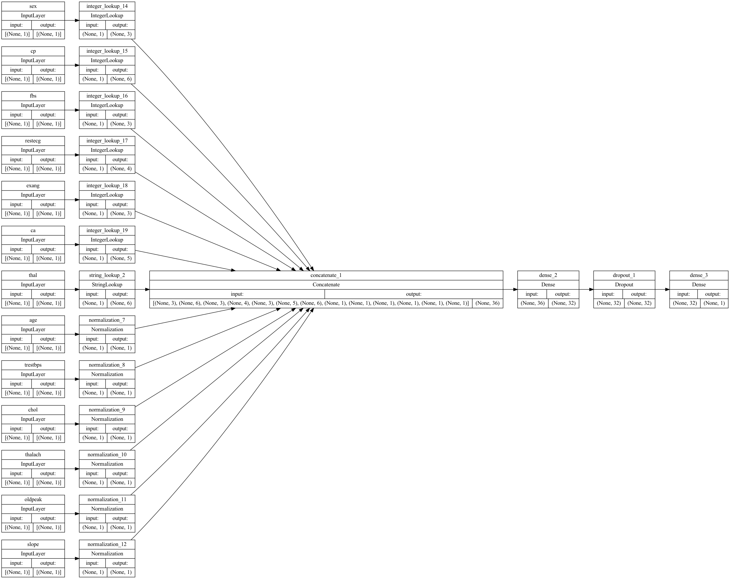
Let’s visualize our connectivity graph:

# `rankdir='LR'` is to make the graph horizontal.
tf.keras.utils.plot_model(model, show_shapes=True, rankdir="LR")

../_images/structured_data_classification_intro_81_0.png

Training#

Next, we train the model for a fixed number of epochs (iterations on a dataset).
An epoch is an arbitrary cutoff, generally defined as “one pass over the entire dataset”, used to separate training into distinct phases, which is useful for logging and periodic evaluation.
Here, we only use 10 epochs.

model.fit(ds_train, epochs=10, validation_data=ds_val)

Epoch 1/10
8/8 [==============================] - 1s 29ms/step - loss: 0.7005 - accuracy: 0.6033 - val_loss: 0.6359 - val_accuracy: 0.7213
Epoch 2/10
8/8 [==============================] - 0s 3ms/step - loss: 0.6558 - accuracy: 0.6777 - val_loss: 0.6018 - val_accuracy: 0.7541
Epoch 3/10
8/8 [==============================] - 0s 3ms/step - loss: 0.6192 - accuracy: 0.6860 - val_loss: 0.5747 - val_accuracy: 0.7705
Epoch 4/10
8/8 [==============================] - 0s 3ms/step - loss: 0.5884 - accuracy: 0.6942 - val_loss: 0.5516 - val_accuracy: 0.7705
Epoch 5/10
8/8 [==============================] - 0s 4ms/step - loss: 0.5947 - accuracy: 0.7397 - val_loss: 0.5297 - val_accuracy: 0.7705
Epoch 6/10
8/8 [==============================] - 0s 3ms/step - loss: 0.5420 - accuracy: 0.7397 - val_loss: 0.5115 - val_accuracy: 0.7705
Epoch 7/10
8/8 [==============================] - 0s 3ms/step - loss: 0.5193 - accuracy: 0.7603 - val_loss: 0.4953 - val_accuracy: 0.7869
Epoch 8/10
8/8 [==============================] - 0s 3ms/step - loss: 0.5153 - accuracy: 0.7397 - val_loss: 0.4811 - val_accuracy: 0.7869
Epoch 9/10
8/8 [==============================] - 0s 3ms/step - loss: 0.4999 - accuracy: 0.7397 - val_loss: 0.4670 - val_accuracy: 0.7541
Epoch 10/10
8/8 [==============================] - 0s 3ms/step - loss: 0.4858 - accuracy: 0.7645 - val_loss: 0.4546 - val_accuracy: 0.7705

<keras.callbacks.History at 0x7fd1ab66a190>

We quickly get to around 80% validation accuracy.

loss, accuracy = model.evaluate(ds_val, verbose=0)

print("Accuracy", round(accuracy, 2))

Accuracy 0.77

Perform inference#

To get a prediction for a new sample, you can simply call model.predict().
There are just two things you need to do:
1. wrap scalars into a list so as to have a batch dimension (models only process batches of data, not single samples)
2. Call convert_to_tensor on each feature

sample = {
    "age": 60,
    "sex": 1,
    "cp": 1,
    "trestbps": 145,
    "chol": 233,
    "fbs": 1,
    "restecg": 2,
    "thalach": 150,
    "exang": 0,
    "oldpeak": 2.3,
    "slope": 3,
    "ca": 0,
    "thal": "fixed",
}

input_dict = {name: tf.convert_to_tensor([value]) for name, value in sample.items()}

predictions = model.predict(input_dict)

print(
    "This particular patient had a %.1f percent probability "
    "of having a heart disease, as evaluated by our model." % (100 * predictions[0][0],)
)

This particular patient had a 42.2 percent probability of having a heart disease, as evaluated by our model.

Next steps#

In this example, we used a lot of code to demonstrate the data preprocessing as simple as possible.
If you want to learn more about how to reduce this code by using functions, take a look at the following example which uses the same data and model: Classification II

Deep Learning

Classification I

Contents

Classification I#

Setup#

Data#

Data import#

Data splitting#

Transform to Tensors#

Examples#

Transformation function#

Use transformation function#

Feature preprocessing#

Categorical features#

Numeric features#

Numerical preprocessing functions#

Categorical preprocessing functions#

Data preprocessing#

Model#

Training#

Perform inference#

Next steps#