SHAP with structured data classification

Explainable AI with TensorFlow, Keras and SHAP

This code tutorial is mainly based on the Keras tutorial “Structured data classification from scratch” by François Chollet and “Census income classification with Keras” by Scott Lundberg.

• To keep this tutorial simple, we will only use numerical features in our binary classification example.

• Take a look at Structured data classification II to see an example of how to use more advanced Keras data preprocessing layers.

Setup

import numpy as np
import pandas as pd

import tensorflow as tf
from tensorflow.keras import layers

from sklearn.model_selection import train_test_split
from sklearn.preprocessing import StandardScaler

import shap

tf.__version__

'2.8.1'

# print the JS visualization code to the notebook
shap.initjs()

Data

Here’s the description of the data:

Column	Description	Feature Type
Age	Age in years	Numerical
Sex	(1 = male; 0 = female)	Categorical
CP	Chest pain type (0, 1, 2, 3, 4)	Categorical
Trestbpd	Resting blood pressure (in mm Hg on admission)	Numerical
Chol	Serum cholesterol in mg/dl	Numerical
FBS	fasting blood sugar in 120 mg/dl (1 = true; 0 = false)	Categorical
RestECG	Resting electrocardiogram results (0, 1, 2)	Categorical
Thalach	Maximum heart rate achieved	Numerical
Exang	Exercise induced angina (1 = yes; 0 = no)	Categorical
Oldpeak	ST depression induced by exercise relative to rest	Numerical
Slope	Slope of the peak exercise ST segment	Numerical
CA	Number of major vessels (0-3) colored by fluoroscopy	Both numerical & categorical
Thal	normal; fixed defect; reversible defect	Categorical (string)
Target	Diagnosis of heart disease (1 = true; 0 = false)	Target

We will only use the following continuous numerical features to predict the variable “Target” (diagnosis of heart disease):

• age

• trestbps

• chol

• thalach

• oldpeak

• slope

Data import

• Let’s download the data and load it into a Pandas dataframe:

file_url = "http://storage.googleapis.com/download.tensorflow.org/data/heart.csv"
df = pd.read_csv(file_url)

Data preparation

# make target variable
y = df.pop('target')

# prepare features
list_numerical = ['age', 'thalach', 'trestbps',  'chol', 'oldpeak']

X = df[list_numerical]

Data splitting

• Let’s split the data into a training and test set

X_train, X_test, y_train, y_test = train_test_split(X, y, test_size=0.2, random_state=42)

Feature preprocessing

scaler = StandardScaler().fit(X_train[list_numerical]) 

X_train[list_numerical] = scaler.transform(X_train[list_numerical])
X_test[list_numerical] = scaler.transform(X_test[list_numerical])

Model

Now we can build the model using the Keras sequential API:

model = tf.keras.Sequential([
    tf.keras.layers.Dense(10, activation='relu'),
    tf.keras.layers.Dense(10, activation='relu'),
    tf.keras.layers.Dense(1, activation='sigmoid')
  ])

model.compile(optimizer="adam", 
              loss ="binary_crossentropy", 
              metrics=["accuracy"])

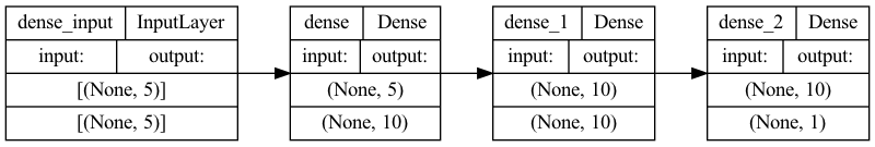
Let’s visualize our connectivity graph:

model.fit(X_train, y_train, 
         epochs=15, 
         batch_size=13,
         validation_data=(X_test, y_test)
         )

Epoch 1/15
 1/19 [>.............................] - ETA: 2s - loss: 0.7202 - accuracy: 0.2308

2022-06-17 21:27:28.476252: W tensorflow/core/platform/profile_utils/cpu_utils.cc:128] Failed to get CPU frequency: 0 Hz

19/19 [==============================] - 0s 4ms/step - loss: 0.7119 - accuracy: 0.3967 - val_loss: 0.7118 - val_accuracy: 0.4754
Epoch 2/15
19/19 [==============================] - 0s 1ms/step - loss: 0.6848 - accuracy: 0.5124 - val_loss: 0.6894 - val_accuracy: 0.4590
Epoch 3/15
19/19 [==============================] - 0s 1ms/step - loss: 0.6650 - accuracy: 0.6157 - val_loss: 0.6705 - val_accuracy: 0.6557
Epoch 4/15
19/19 [==============================] - 0s 1ms/step - loss: 0.6477 - accuracy: 0.6818 - val_loss: 0.6566 - val_accuracy: 0.6885
Epoch 5/15
19/19 [==============================] - 0s 1ms/step - loss: 0.6311 - accuracy: 0.7397 - val_loss: 0.6434 - val_accuracy: 0.7377
Epoch 6/15
19/19 [==============================] - 0s 1ms/step - loss: 0.6161 - accuracy: 0.7479 - val_loss: 0.6301 - val_accuracy: 0.7377
Epoch 7/15
19/19 [==============================] - 0s 1ms/step - loss: 0.6015 - accuracy: 0.7893 - val_loss: 0.6170 - val_accuracy: 0.7377
Epoch 8/15
19/19 [==============================] - 0s 1ms/step - loss: 0.5857 - accuracy: 0.7975 - val_loss: 0.6058 - val_accuracy: 0.7377
Epoch 9/15
19/19 [==============================] - 0s 975us/step - loss: 0.5714 - accuracy: 0.8017 - val_loss: 0.5969 - val_accuracy: 0.7377
Epoch 10/15
19/19 [==============================] - 0s 990us/step - loss: 0.5581 - accuracy: 0.7975 - val_loss: 0.5867 - val_accuracy: 0.7705
Epoch 11/15
19/19 [==============================] - 0s 1ms/step - loss: 0.5412 - accuracy: 0.7934 - val_loss: 0.5783 - val_accuracy: 0.7869
Epoch 12/15
19/19 [==============================] - 0s 1ms/step - loss: 0.5260 - accuracy: 0.7893 - val_loss: 0.5705 - val_accuracy: 0.7869
Epoch 13/15
19/19 [==============================] - 0s 1ms/step - loss: 0.5121 - accuracy: 0.7934 - val_loss: 0.5637 - val_accuracy: 0.7705
Epoch 14/15
19/19 [==============================] - 0s 1ms/step - loss: 0.4980 - accuracy: 0.8058 - val_loss: 0.5581 - val_accuracy: 0.7869
Epoch 15/15
19/19 [==============================] - 0s 1ms/step - loss: 0.4860 - accuracy: 0.8099 - val_loss: 0.5534 - val_accuracy: 0.7869

<keras.callbacks.History at 0x1667baad0>

# `rankdir='LR'` is to make the graph horizontal.
tf.keras.utils.plot_model(model, show_shapes=True, rankdir="LR")

loss, accuracy = model.evaluate(X_test, y_test)

print("Accuracy", accuracy)

2/2 [==============================] - 0s 1ms/step - loss: 0.5534 - accuracy: 0.7869
Accuracy 0.7868852615356445

Perform inference

• Let’s save the heart diseases classification model to demonstrate the process of a real world scenario (where we would first save the model and reload it in a different production environment):

model.save('classifier_hd')

INFO:tensorflow:Assets written to: classifier_hd/assets

2022-06-12 17:01:00.553972: W tensorflow/python/util/util.cc:368] Sets are not currently considered sequences, but this may change in the future, so consider avoiding using them.

• Load the model:

reloaded_model = tf.keras.models.load_model('classifier_hd')

predictions = reloaded_model.predict(X_train)

print(
    "This particular patient had a %.1f percent probability "
    "of having a heart disease, as evaluated by our model." % (100 * predictions[0][0],)
)

This particular patient had a 24.8 percent probability of having a heart disease, as evaluated by our model.

SHAP

We use our model and a selection of 50 samples from the dataset to represent “typical” feature values (the so called background distribution).

explainer = shap.KernelExplainer(model, X_train.iloc[:50,:])

Now we use 500 perterbation samples to estimate the SHAP values for a given prediction (at index location 20). Note that this requires 500 * 50 evaluations of the model.

shap_values = explainer.shap_values(X_train.iloc[20,:], nsamples=500)

The so called force plot below shows how each feature contributes to push the model output from the base value (the average model output over the training dataset we passed) to the model output. Features pushing the prediction higher are shown in red, those pushing the prediction lower are in blue. To learn more about force plots, take a look at this Nature BME paper from Lundberg et al. (2018).

shap.force_plot(explainer.expected_value, shap_values[0], X_train.iloc[20,:])

Visualization omitted, Javascript library not loaded!
Have you run `initjs()` in this notebook? If this notebook was from another user you must also trust this notebook (File -> Trust notebook). If you are viewing this notebook on github the Javascript has been stripped for security. If you are using JupyterLab this error is because a JupyterLab extension has not yet been written.

Explain many predictions

If we take many force plot explanations such as the one shown above, rotate them 90 degrees, and then stack them horizontally, we can see explanations for an entire dataset (see content below). Here, we repeat the above explanation process for 50 individuals.

To understand how a single feature effects the output of the model we can plot the SHAP value of that feature vs. the value of the feature for all the examples in a dataset. Since SHAP values represent a feature’s responsibility for a change in the model output, the plot below represents the change in the dependent variable. Vertical dispersion at a single value of represents interaction effects with other features.

shap_values50 = explainer.shap_values(X_train.iloc[50:100,:], nsamples=500)

shap.force_plot(explainer.expected_value, shap_values50[0], X_train.iloc[50:100,:])

Visualization omitted, Javascript library not loaded!
Have you run `initjs()` in this notebook? If this notebook was from another user you must also trust this notebook (File -> Trust notebook). If you are viewing this notebook on github the Javascript has been stripped for security. If you are using JupyterLab this error is because a JupyterLab extension has not yet been written.