Machine Learning project#

This notebook is a short version of the end-to-end Machine Learning project provided by Aurélien Geron.

Setup#

This project requires:

Python 3.7 or above
Scikit-Learn ≥ 1.0.1:

%matplotlib inline

import sys
from pathlib import Path

import numpy as np
import pandas as pd
from pandas.plotting import scatter_matrix
import matplotlib.pyplot as plt

import sklearn
from sklearn import set_config
set_config(display='diagram')

plt.rc('font', size=14)
plt.rc('axes', labelsize=14, titlesize=14)
plt.rc('legend', fontsize=14)
plt.rc('xtick', labelsize=10)
plt.rc('ytick', labelsize=10)

# Check if you have the correct versions
assert sklearn.__version__ >= "1.0.1"
assert sys.version_info >= (3, 7)

Data#

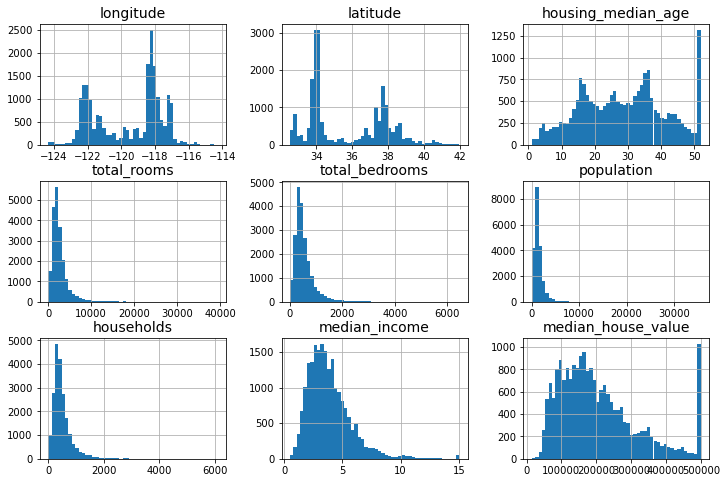
Welcome to Machine Learning Housing Corp.! Your task is to predict median house values in Californian districts, given a number of features from these districts.

housing = pd.read_csv("https://raw.githubusercontent.com/kirenz/datasets/master/housing_hml3.csv")

Overview#

housing.head()

	longitude	latitude	housing_median_age	total_rooms	total_bedrooms	population	households	median_income	median_house_value	ocean_proximity
0	-122.23	37.88	41.0	880.0	129.0	322.0	126.0	8.3252	452600.0	NEAR BAY
1	-122.22	37.86	21.0	7099.0	1106.0	2401.0	1138.0	8.3014	358500.0	NEAR BAY
2	-122.24	37.85	52.0	1467.0	190.0	496.0	177.0	7.2574	352100.0	NEAR BAY
3	-122.25	37.85	52.0	1274.0	235.0	558.0	219.0	5.6431	341300.0	NEAR BAY
4	-122.25	37.85	52.0	1627.0	280.0	565.0	259.0	3.8462	342200.0	NEAR BAY

housing.info()

<class 'pandas.core.frame.DataFrame'>
RangeIndex: 20640 entries, 0 to 20639
Data columns (total 10 columns):
 #   Column              Non-Null Count  Dtype  
---  ------              --------------  -----  
 0   longitude           20640 non-null  float64
 1   latitude            20640 non-null  float64
 2   housing_median_age  20640 non-null  float64
 3   total_rooms         20640 non-null  float64
 4   total_bedrooms      20433 non-null  float64
 5   population          20640 non-null  float64
 6   households          20640 non-null  float64
 7   median_income       20640 non-null  float64
 8   median_house_value  20640 non-null  float64
 9   ocean_proximity     20640 non-null  object 
dtypes: float64(9), object(1)
memory usage: 1.6+ MB

housing["ocean_proximity"].value_counts()

<1H OCEAN     7274
INLAND        5301
NEAR OCEAN    2089
NEAR BAY      1846
ISLAND           2
Name: ocean_proximity, dtype: int64

housing.describe().T

	count	mean	std	min	25%	50%	75%	max
longitude	16512.0	-119.573125	2.000624	-124.3500	-121.8000	-118.5100	-118.01	-114.4900
latitude	16512.0	35.637746	2.133294	32.5500	33.9300	34.2600	37.72	41.9500
housing_median_age	16512.0	28.577156	12.585738	1.0000	18.0000	29.0000	37.00	52.0000
total_rooms	16512.0	2639.402798	2185.287466	2.0000	1447.0000	2125.0000	3154.00	39320.0000
total_bedrooms	16344.0	538.949094	423.862079	1.0000	296.0000	434.0000	645.00	6210.0000
population	16512.0	1425.513929	1094.795467	3.0000	787.0000	1167.0000	1726.00	16305.0000
households	16512.0	499.990189	382.865787	1.0000	279.0000	408.0000	603.00	5358.0000
median_income	16512.0	3.870428	1.891936	0.4999	2.5625	3.5385	4.75	15.0001

housing.hist(bins=50, figsize=(12, 8));

Data split#

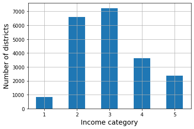
housing["income_cat"] = pd.cut(housing["median_income"],
                               bins=[0., 1.5, 3.0, 4.5, 6., np.inf],
                               labels=[1, 2, 3, 4, 5])

housing["income_cat"].value_counts().sort_index().plot.bar(rot=0, grid=True)

plt.xlabel("Income category")
plt.ylabel("Number of districts");

Stratified split:

from sklearn.model_selection import train_test_split

strat_train_set, strat_test_set = train_test_split(
    housing, test_size=0.2, stratify=housing["income_cat"], random_state=42)

Drop the variable “income_cat” from our datasets:

for set_ in (strat_train_set, strat_test_set):
    set_.drop("income_cat", axis=1, inplace=True)

Exploration#

housing = strat_train_set.copy()

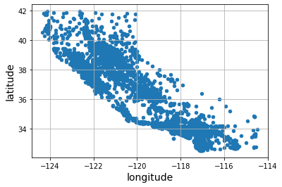
Visualizing Geographical Data#

housing.plot(kind="scatter", x="longitude", y="latitude", grid=True);

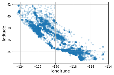
housing.plot(kind="scatter", x="longitude", y="latitude", grid=True, alpha=0.2);

housing.plot(kind="scatter", 
             x="longitude", 
             y="latitude", 
             grid=True,
             s=housing["population"] / 100, 
             label="population",
             c="median_house_value", 
             cmap="jet", 
             colorbar=True,
             legend=True, 
             sharex=False, 
             figsize=(10, 7)
             );

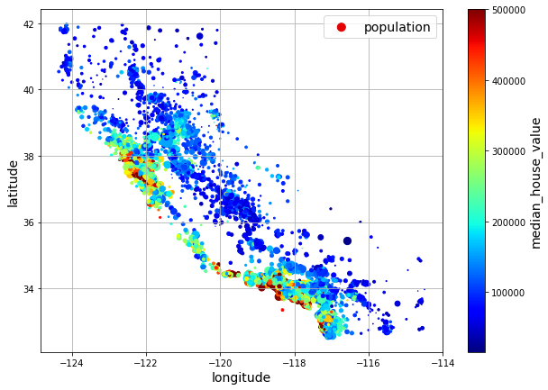
The argument sharex=False fixes a display bug: without it, the x-axis values and label are not displayed (see: https://github.com/pandas-dev/pandas/issues/10611).

Correlations#

corr_matrix = housing.corr()

corr_matrix["median_house_value"].sort_values(ascending=False)

median_house_value    1.000000
median_income         0.688380
total_rooms           0.137455
housing_median_age    0.102175
households            0.071426
total_bedrooms        0.054635
population           -0.020153
longitude            -0.050859
latitude             -0.139584
Name: median_house_value, dtype: float64

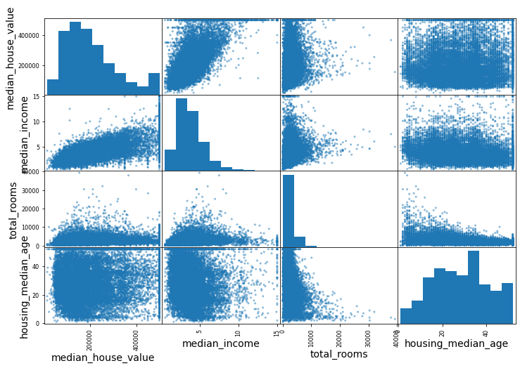
attributes = ["median_house_value", "median_income", "total_rooms", "housing_median_age"]

scatter_matrix(housing[attributes], figsize=(12, 8));

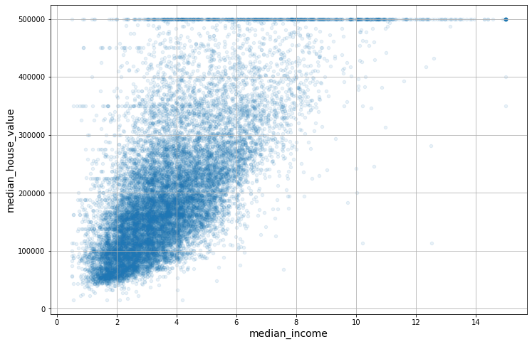
housing.plot(kind="scatter", 
             x="median_income", 
             y="median_house_value",
             alpha=0.1, 
             grid=True,
             figsize=(12, 8));

Feature Engineering#

Experimenting with Attribute Combinations

housing["rooms_per_house"] = housing["total_rooms"] / housing["households"]
housing["bedrooms_ratio"] = housing["total_bedrooms"] / housing["total_rooms"]
housing["people_per_house"] = housing["population"] / housing["households"]

corr_matrix = housing.corr()
corr_matrix["median_house_value"].sort_values(ascending=False)

median_house_value    1.000000
median_income         0.688380
rooms_per_house       0.143663
total_rooms           0.137455
housing_median_age    0.102175
households            0.071426
total_bedrooms        0.054635
population           -0.020153
people_per_house     -0.038224
longitude            -0.050859
latitude             -0.139584
bedrooms_ratio       -0.256397
Name: median_house_value, dtype: float64

Data Pipeline#

Let’s revert to the original training set and separate the target (note that strat_train_set.drop() creates a copy of strat_train_set without the column, it doesn’t actually modify strat_train_set itself, unless you pass inplace=True):

housing = strat_train_set.drop("median_house_value", axis=1)

housing_labels = strat_train_set["median_house_value"].copy()

Now let’s build a pipeline to preprocess the attributes:

num_attribs = ["longitude", "latitude", "housing_median_age", "total_rooms",
               "total_bedrooms", "population", "households", "median_income"]
               
cat_attribs = ["ocean_proximity"]

from sklearn.pipeline import make_pipeline
from sklearn.impute import SimpleImputer
from sklearn.preprocessing import OneHotEncoder

# categorical pipeline
cat_pipeline = make_pipeline(
    SimpleImputer(strategy="most_frequent"),
    OneHotEncoder(handle_unknown="ignore")
    )

# default numerical pipeline
from sklearn.preprocessing import StandardScaler

default_num_pipeline = make_pipeline(
    SimpleImputer(strategy="median"),
    StandardScaler()
    )

# custom function to make ratios
def column_ratio(X):
    return X[:, [0]] / X[:, [1]]

from sklearn.preprocessing import FunctionTransformer
from sklearn.preprocessing import StandardScaler

# custom function to transfomr ratios
def ratio_pipeline(name=None):
    return make_pipeline(
        SimpleImputer(strategy="median"),
        FunctionTransformer(column_ratio),
        StandardScaler())

# custom log transformer
log_pipeline = make_pipeline(
    SimpleImputer(strategy="median"),
    FunctionTransformer(np.log),
    StandardScaler())

To learn more about developing scikit-learn estimators, take a look at this page
Here is a template to build your own scikit-learn functions: template

# custom cluster similarity  
from sklearn.cluster import KMeans
from sklearn.base import BaseEstimator, TransformerMixin
from sklearn.metrics.pairwise import rbf_kernel


class ClusterSimilarity(BaseEstimator, TransformerMixin):
    def __init__(self, n_clusters=10, gamma=1.0, random_state=None):
        self.n_clusters = n_clusters
        self.gamma = gamma
        self.random_state = random_state

    def fit(self, X, y=None, sample_weight=None):
        self.kmeans_ = KMeans(self.n_clusters, random_state=self.random_state)
        self.kmeans_.fit(X, sample_weight=sample_weight)
        return self  # always return self!

    def transform(self, X):
        return rbf_kernel(X, self.kmeans_.cluster_centers_, gamma=self.gamma)
    
    def get_feature_names_out(self, names=None):
        return [f"Cluster {i} similarity" for i in range(self.n_clusters)]

# custom cluster similarity step 
cluster_simil = ClusterSimilarity(n_clusters=10, gamma=1., random_state=42)

Perform transformations:

from sklearn.compose import ColumnTransformer
from sklearn.compose import make_column_selector


preprocessing = ColumnTransformer([
        ("bedrooms_ratio", ratio_pipeline("bedrooms_ratio"),
                           ["total_bedrooms", "total_rooms"]),

        ("rooms_per_house", ratio_pipeline("rooms_per_house"),
                            ["total_rooms", "households"]),

        ("people_per_house", ratio_pipeline("people_per_house"),
                             ["population", "households"]),

        ("log", log_pipeline, ["total_bedrooms", "total_rooms",
                               "population", "households", "median_income"]),

        ("geo", cluster_simil, ["latitude", "longitude"]),
        
        ("cat", cat_pipeline, make_column_selector(dtype_include=object)),
    ],
    remainder=default_num_pipeline)  # one column remaining: housing_median_age

housing_prepared = preprocessing.fit_transform(housing)

housing_prepared.shape

(16512, 24)

Cross-Validation#

Decision Tree#

from sklearn.model_selection import cross_val_score

# we only use cv=3 instead of cv=10 to speed up the computation
tree_rmses = -cross_val_score(tree_reg, housing, housing_labels,
                              scoring="neg_root_mean_squared_error", cv=3)

pd.Series(tree_rmses).describe()

count        3.000000
mean     68282.891053
std       1486.492256
min      66810.075215
25%      67532.990434
50%      68255.905652
75%      69019.298971
max      69782.692291
dtype: float64

Linear Regression#

lin_rmses = -cross_val_score(lin_reg, housing, housing_labels,
                              scoring="neg_root_mean_squared_error", cv=3)

pd.Series(lin_rmses).describe()

count        3.000000
mean     69778.756842
std       1629.907725
min      67980.530959
25%      69088.686886
50%      70196.842814
75%      70677.869784
max      71158.896754
dtype: float64

Random Forest#

Again, we set cv=3 instead of cv=10:

from sklearn.ensemble import RandomForestRegressor

forest_reg = make_pipeline(preprocessing,
                           RandomForestRegressor(random_state=42))
                           
forest_rmses = -cross_val_score(forest_reg, housing, housing_labels,
                                scoring="neg_root_mean_squared_error", cv=3)

pd.Series(forest_rmses).describe()

count        3.000000
mean     47889.465303
std        619.080587
min      47392.624982
25%      47542.700149
50%      47692.775316
75%      48137.885464
max      48582.995613
dtype: float64

Let’s compare this RMSE measured using cross-validation (the “validation error”) with the RMSE measured on the training set (the “training error”):

forest_reg.fit(housing, housing_labels)

housing_predictions = forest_reg.predict(housing)

forest_rmse = mean_squared_error(housing_labels, housing_predictions,
                                 squared=False)
forest_rmse

17474.619286483998

The training error is much lower than the validation error, which usually means that the model has overfit the training set. Another possible explanation may be that there’s a mismatch between the training data and the validation data, but it’s not the case here, since both came from the same dataset that we shuffled and split in two parts.

Fine-Tuning#

Grid Search#

from sklearn.model_selection import GridSearchCV
from sklearn.pipeline import Pipeline

full_pipeline = Pipeline([
    ("preprocessing", preprocessing),
    ("random_forest", RandomForestRegressor(random_state=42)),
])

param_grid = [
    {'preprocessing__geo__n_clusters': [5, 8, 10],
     'random_forest__max_features': [4, 6, 8]},
    {'preprocessing__geo__n_clusters': [10, 15],
     'random_forest__max_features': [6, 8, 10]},
]

grid_search = GridSearchCV(full_pipeline, param_grid, cv=3,
                           scoring='neg_root_mean_squared_error')

Warning: the following cell may take a few minutes to run:

You can get the full list of hyperparameters available for tuning by looking at full_pipeline.get_params().keys():

# extra code – shows part of the output of get_params().keys()
print(str(full_pipeline.get_params().keys())[:1000] + "...")

dict_keys(['memory', 'steps', 'verbose', 'preprocessing', 'random_forest', 'preprocessing__n_jobs', 'preprocessing__remainder__memory', 'preprocessing__remainder__steps', 'preprocessing__remainder__verbose', 'preprocessing__remainder__simpleimputer', 'preprocessing__remainder__standardscaler', 'preprocessing__remainder__simpleimputer__add_indicator', 'preprocessing__remainder__simpleimputer__copy', 'preprocessing__remainder__simpleimputer__fill_value', 'preprocessing__remainder__simpleimputer__missing_values', 'preprocessing__remainder__simpleimputer__strategy', 'preprocessing__remainder__simpleimputer__verbose', 'preprocessing__remainder__standardscaler__copy', 'preprocessing__remainder__standardscaler__with_mean', 'preprocessing__remainder__standardscaler__with_std', 'preprocessing__remainder', 'preprocessing__sparse_threshold', 'preprocessing__transformer_weights', 'preprocessing__transformers', 'preprocessing__verbose', 'preprocessing__verbose_feature_names_out', 'preprocessing__be...

The best hyperparameter combination found:

grid_search.best_params_

{'preprocessing__geo__n_clusters': 15, 'random_forest__max_features': 6}

Let’s look at the score of each hyperparameter combination tested during the grid search:

cv_res = pd.DataFrame(grid_search.cv_results_)

cv_res.sort_values(by="mean_test_score", ascending=False, inplace=True)

# extra code – these few lines of code just make the DataFrame look nicer
cv_res = cv_res[["param_preprocessing__geo__n_clusters",
                 "param_random_forest__max_features", "split0_test_score",
                 "split1_test_score", "split2_test_score", "mean_test_score"]]

score_cols = ["split0", "split1", "split2", "mean_test_rmse"]

cv_res.columns = ["n_clusters", "max_features"] + score_cols

cv_res[score_cols] = -cv_res[score_cols].round().astype(np.int64)

cv_res.head()

	n_clusters	max_features	split0	split1	split2	mean_test_rmse
12	15	6	43460	43919	44748	44042
13	15	8	44132	44075	45010	44406
14	15	10	44374	44286	45316	44659
7	10	6	44683	44655	45657	44999
9	10	6	44683	44655	45657	44999

Randomized Search#

from sklearn.experimental import enable_halving_search_cv
from sklearn.model_selection import HalvingRandomSearchCV

Warning: the following cell may take a few minutes to run:

Try 30 (n_iter × cv) random combinations of hyperparameters:

# extra code – displays the random search results
cv_res = pd.DataFrame(rnd_search.cv_results_)

cv_res.sort_values(by="mean_test_score", ascending=False, inplace=True)

cv_res = cv_res[["param_preprocessing__geo__n_clusters",
                 "param_random_forest__max_features", "split0_test_score",
                 "split1_test_score", "split2_test_score", "mean_test_score"]]

cv_res.columns = ["n_clusters", "max_features"] + score_cols

cv_res[score_cols] = -cv_res[score_cols].round().astype(np.int64)

cv_res.head()

	n_clusters	max_features	split0	split1	split2	mean_test_rmse
0	9	5	45311	44727	46099	45379
4	9	3	45721	45397	46743	45953
7	7	5	45887	45597	46504	45996
3	7	6	45633	45815	46702	46050
1	7	8	45887	45820	46809	46172

Analyze Errors#

Analyze Errors of Best Model

final_model = rnd_search.best_estimator_  # includes preprocessing

feature_importances = final_model["random_forest"].feature_importances_

feature_importances.round(2)

array([0.08, 0.06, 0.08, 0.01, 0.01, 0.01, 0.01, 0.25, 0.04, 0.03, 0.04,
       0.03, 0.04, 0.06, 0.02, 0.03, 0.02, 0.01, 0.12, 0.  , 0.  , 0.01,
       0.03])

Evaluate on Test Set#

X_test = strat_test_set.drop("median_house_value", axis=1)
y_test = strat_test_set["median_house_value"].copy()

final_predictions = final_model.predict(X_test)

final_rmse = mean_squared_error(y_test, final_predictions, squared=False)
print(final_rmse)

44556.01747258438

We can compute a 95% confidence interval for the test RMSE:

from scipy import stats

confidence = 0.95

squared_errors = (final_predictions - y_test) ** 2

np.sqrt(stats.t.interval(confidence, len(squared_errors) - 1,
                         loc=squared_errors.mean(),
                         scale=stats.sem(squared_errors)))

array([42373.48736315, 46636.51953908])

Save model#

Model persistence using joblib

Save the final model:

import joblib

joblib.dump(final_model, "my_california_housing_model.pkl")

['my_california_housing_model.pkl']

Now you can deploy this model to production. For example, the following code could be a script that would run in production:

final_model_reloaded = joblib.load("my_california_housing_model.pkl")

new_data = housing.iloc[:5]  # pretend these are new districts

predictions = final_model_reloaded.predict(new_data)

predictions

array([429545.11      , 462980.09      , 108348.47761194,  99628.        ,
       345977.07      ])

Introduction to Regression Models

Machine Learning project

Contents

Machine Learning project#

Setup#

Data#

Overview#

Data split#

Exploration#

Visualizing Geographical Data#

Correlations#

Feature Engineering#

Data Pipeline#

Models#

Linear Regression#

Decision Tree#

Cross-Validation#

Decision Tree#

Linear Regression#

Random Forest#

Fine-Tuning#

Grid Search#

Randomized Search#

Analyze Errors#

Evaluate on Test Set#

Save model#

Exercise solutions#

1. Support Vector Machine#

2. Randomized Search CV#

3. SelectFromModel#