Simple statsmodels model

Does money make people happier? Simple version without data splitting.

Data preparation

import pandas as pd

# Load the data from GitHub
LINK = "https://raw.githubusercontent.com/kirenz/datasets/master/oecd_gdp.csv"
df = pd.read_csv(LINK)

df.head()

	Country	GDP per capita	Life satisfaction
0	Russia	9054.914	6.0
1	Turkey	9437.372	5.6
2	Hungary	12239.894	4.9
3	Poland	12495.334	5.8
4	Slovak Republic	15991.736	6.1

df.info()

<class 'pandas.core.frame.DataFrame'>
RangeIndex: 29 entries, 0 to 28
Data columns (total 3 columns):
 #   Column             Non-Null Count  Dtype  
---  ------             --------------  -----  
 0   Country            29 non-null     object 
 1   GDP per capita     29 non-null     float64
 2   Life satisfaction  29 non-null     float64
dtypes: float64(2), object(1)
memory usage: 824.0+ bytes

# Change column names 
df.columns = df.columns.str.lower().str.replace(' ', '_')

df.head()

	country	gdp_per_capita	life_satisfaction
0	Russia	9054.914	6.0
1	Turkey	9437.372	5.6
2	Hungary	12239.894	4.9
3	Poland	12495.334	5.8
4	Slovak Republic	15991.736	6.1

%matplotlib inline
import seaborn as sns

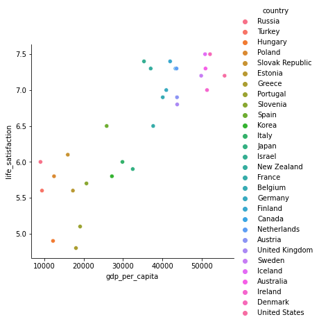
# Visualize the data
sns.relplot(x="gdp_per_capita", y='life_satisfaction', hue='country', data=df);

Simple linear regression model

import statsmodels.formula.api as smf

# Estimate the model 
lm = smf.ols(formula ='life_satisfaction ~ gdp_per_capita', data=df).fit()

# Model coefficients
lm.summary()

OLS Regression Results

Dep. Variable:	life_satisfaction	R-squared:	0.734
Model:	OLS	Adj. R-squared:	0.725
Method:	Least Squares	F-statistic:	74.67
Date:	Wed, 16 Mar 2022	Prob (F-statistic):	2.95e-09
Time:	16:53:19	Log-Likelihood:	-16.345
No. Observations:	29	AIC:	36.69
Df Residuals:	27	BIC:	39.42
Df Model:	1
Covariance Type:	nonrobust

	coef	std err	t	P>|t|	[0.025	0.975]
Intercept	4.8531	0.207	23.481	0.000	4.429	5.277
gdp_per_capita	4.912e-05	5.68e-06	8.641	0.000	3.75e-05	6.08e-05

Omnibus:	0.308	Durbin-Watson:	1.454
Prob(Omnibus):	0.857	Jarque-Bera (JB):	0.486
Skew:	-0.094	Prob(JB):	0.784
Kurtosis:	2.394	Cond. No.	9.19e+04

Notes:
[1] Standard Errors assume that the covariance matrix of the errors is correctly specified.
[2] The condition number is large, 9.19e+04. This might indicate that there are
strong multicollinearity or other numerical problems.

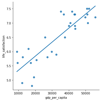
# Plot regression line 
sns.lmplot(data=df, x="gdp_per_capita", y="life_satisfaction", ci=False);

# Add the regression predictions (as "pred") to our DataFrame
df['y_pred'] = lm.predict(df.gdp_per_capita)

from statsmodels.tools.eval_measures import mse, rmse

# Performance measures

# MSE
mse(df['life_satisfaction'], df['y_pred'])

0.18075033705835147

# RMSE
rmse(df['life_satisfaction'], df['y_pred'])

0.42514742979153886