Scikit-learn

In this tutorial, we will build a model with the Python scikit-learn module. Additionally, you will learn how to create a data preprocessing pipline.

Data preparation

# See section "Data" for details about data preprocessing
from case_duke_data_prep import *

Data preprocessing pipeline

# Modules
from sklearn.compose import ColumnTransformer
from sklearn.compose import make_column_selector as selector
from sklearn.pipeline import Pipeline
from sklearn.impute import SimpleImputer
from sklearn import set_config
from sklearn.preprocessing import StandardScaler, OneHotEncoder

# for numeric features
numeric_transformer = Pipeline(steps=[
    ('imputer', SimpleImputer(strategy='median')),
    ('scaler', StandardScaler())
    ])

# for categorical features  
categorical_transformer = Pipeline(steps=[
    ('imputer', SimpleImputer(strategy='constant', fill_value='missing')),
    ('onehot', OneHotEncoder(handle_unknown='ignore'))
    ])

# Pipeline
preprocessor = ColumnTransformer(transformers=[
    ('num', numeric_transformer, selector(dtype_exclude="category")),
    ('cat', categorical_transformer, selector(dtype_include="category"))
        ])

Simple regression

# Select features for simple regression
features = ['area']
X = df[features]

# Create response
y = df["price"]

# check feature
X.info()

<class 'pandas.core.frame.DataFrame'>
Int64Index: 97 entries, 0 to 97
Data columns (total 1 columns):
 #   Column  Non-Null Count  Dtype
---  ------  --------------  -----
 0   area    97 non-null     int64
dtypes: int64(1)
memory usage: 1.5 KB

# check label
y

0     1520000
1     1030000
2      420000
3      680000
4      428500
       ...   
93     541000
94     473000
95     490000
96     815000
97     674500
Name: price, Length: 97, dtype: int64

# check for missing values
print("Missing values X:",X.isnull().any(axis=1).sum())

print("Missing values Y:",y.isnull().sum())

Missing values X: 0
Missing values Y: 0

Data splitting

from sklearn.model_selection import train_test_split

# Train Test Split
# Use random_state to make this notebook's output identical at every run
X_train, X_test, y_train, y_test = train_test_split(X, y, test_size=0.2, random_state=42)

Modeling

from sklearn.linear_model import LinearRegression

# Create pipeline with model
lm_pipe = Pipeline(steps=[
    ('preprocessor', preprocessor),
    ('lm', LinearRegression())
                        ])

# show pipeline
set_config(display="diagram")
# Fit model
lm_pipe.fit(X_train, y_train)

Pipeline(steps=[('preprocessor',
                 ColumnTransformer(transformers=[('num',
                                                  Pipeline(steps=[('imputer',
                                                                   SimpleImputer(strategy='median')),
                                                                  ('scaler',
                                                                   StandardScaler())]),
                                                  <sklearn.compose._column_transformer.make_column_selector object at 0x7fd057eb4a30>),
                                                 ('cat',
                                                  Pipeline(steps=[('imputer',
                                                                   SimpleImputer(fill_value='missing',
                                                                                 strategy='constant')),
                                                                  ('onehot',
                                                                   OneHotEncoder(handle_unknown='ignore'))]),
                                                  <sklearn.compose._column_transformer.make_column_selector object at 0x7fd058f4dbe0>)])),
                ('lm', LinearRegression())])

Please rerun this cell to show the HTML repr or trust the notebook.

# Obtain model coefficients
lm_pipe.named_steps['lm'].coef_

array([128046.72300033])

Evaluation with training data

There are various options to evaluate a model in scikit-learn. Review this overview about metrics and scoring: quantifying the quality of predictions.

X_train.head()

	area
49	2902
71	2165
69	1094
15	2750
39	2334

y_pred = lm_pipe.predict(X_train)

from sklearn.metrics import r2_score

r2_score(y_train, y_pred)  

0.35694914972541525

from sklearn.metrics import mean_squared_error

mean_squared_error(y_train, y_pred)

29537647395.092514

# RMSE
mean_squared_error(y_train, y_pred, squared=False)

171865.20123367765

from sklearn.metrics import mean_absolute_error

mean_absolute_error(y_train, y_pred)

115668.27028304595

%matplotlib inline
import seaborn as sns 
sns.set_theme(style="ticks")

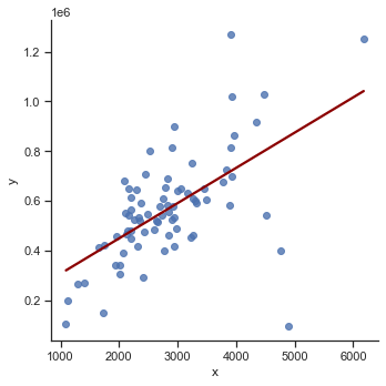
# Plot with Seaborn

# We first need to create a DataFrame
df_train = pd.DataFrame({'x': X_train['area'], 'y':y_train})

sns.lmplot(x='x', y='y', data=df_train, line_kws={'color': 'darkred'}, ci=False);

import plotly.io as pio
import plotly.offline as py
import plotly.express as px

# Plot with Plotly Express
fig = px.scatter(x=X_train['area'], y=y_train, opacity=0.65, 
                trendline='ols', trendline_color_override='darkred');

fig.show()

sns.residplot(x=y_pred, y=y_train, scatter_kws={"s": 80});

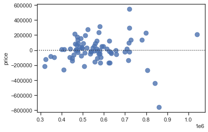
Let’s take a look at the wrongest predictions:

# create dataframe
df_error = pd.DataFrame(
    { "y": y_train,
      "y_pred": y_pred,
      "error": y_pred - y_train
    })

# sort by error, select top 10 and get index
error_index = df_error.sort_values(by=['error']).nlargest(10, 'error').index

# show corresponding data observations
df.iloc[error_index]

	price	bed	bath	area	year_built	cooling	lot
65	609000	5	4.0	3175	2016	other	0.47
84	567000	4	4.0	3931	1982	other	0.39
88	480000	2	2.0	2203	1984	other	0.42
55	150000	3	1.0	1734	1945	other	0.16
19	290000	3	2.5	2414	1956	other	0.48
70	520000	4	3.0	2637	1968	other	0.65
16	452500	3	2.5	3234	1941	other	0.61
92	590000	5	3.0	3323	1980	other	0.43
48	416000	5	3.0	2949	1955	other	0.55
57	400000	4	3.0	2771	1958	central	0.52

Evaluation with test data

y_pred = lm_pipe.predict(X_test)

print('MSE:', mean_squared_error(y_test, y_pred))

print('RMSE:', mean_squared_error(y_test, y_pred, squared=False))

MSE: 23209825917.075768
RMSE: 152347.7138557575

# Plot with Plotly Express
fig = px.scatter(x=X_test['area'], y=y_test, opacity=0.65, 
                trendline='ols', trendline_color_override='darkred')

fig.show()

Model generalization on unseen data (see plotly documentation)

import numpy as np
import plotly.graph_objects as go

x_range = pd.DataFrame({ 'area': np.linspace(X_train['area'].min(), X_train['area'].max(), 100)})
y_range =  lm_pipe.predict(x_range)

go.Figure([
    go.Scatter(x=X_train.squeeze(), y=y_train, name='train', mode='markers'),
    go.Scatter(x=X_test.squeeze(), y=y_test, name='test', mode='markers'),
    go.Scatter(x=x_range.area, y=y_range, name='prediction')
])

Multiple regression

# Select features for multiple regression
features= [
 'bed',
 'bath',
 'area',
 'year_built',
 'cooling',
 'lot'
  ]
X = df[features]

X.info()
print("Missing values:",X.isnull().any(axis = 1).sum())

# Create response
y = df["price"]

<class 'pandas.core.frame.DataFrame'>
Int64Index: 97 entries, 0 to 97
Data columns (total 6 columns):
 #   Column      Non-Null Count  Dtype   
---  ------      --------------  -----   
 0   bed         97 non-null     int64   
 1   bath        97 non-null     float64 
 2   area        97 non-null     int64   
 3   year_built  97 non-null     int64   
 4   cooling     97 non-null     category
 5   lot         97 non-null     float64 
dtypes: category(1), float64(2), int64(3)
memory usage: 4.8 KB
Missing values: 0

# Data splitting
X_train, X_test, y_train, y_test = train_test_split(X, y, test_size=0.2, random_state=42)

# Create pipeline with model
lm_pipe = Pipeline(steps=[
    ('preprocessor', preprocessor),
    ('lm', LinearRegression())
                        ])

# show pipeline
set_config(display="diagram")
# Fit model
lm_pipe.fit(X_train, y_train)

Pipeline(steps=[('preprocessor',
                 ColumnTransformer(transformers=[('num',
                                                  Pipeline(steps=[('imputer',
                                                                   SimpleImputer(strategy='median')),
                                                                  ('scaler',
                                                                   StandardScaler())]),
                                                  <sklearn.compose._column_transformer.make_column_selector object at 0x7fdb7e834040>),
                                                 ('cat',
                                                  Pipeline(steps=[('imputer',
                                                                   SimpleImputer(fill_value='missing',
                                                                                 strategy='constant')),
                                                                  ('onehot',
                                                                   OneHotEncoder(handle_unknown='ignore'))]),
                                                  <sklearn.compose._column_transformer.make_column_selector object at 0x7fdb7e834070>)])),
                ('lm', LinearRegression())])

Please rerun this cell to show the HTML repr or trust the notebook.

# Obtain model coefficients
lm_pipe.named_steps['lm'].coef_

array([ 37501.22436002,  50280.7007969 ,  30312.97805437,  27994.3520344 ,
        79024.39994917,  23467.73502737, -23467.73502737])

Evaluation with test data:

y_pred = lm_pipe.predict(X_test)

r2_score(y_test, y_pred)

0.4825836731448806