Generalized Additive Models (GAM)#

The following code tutorial is mainly based on the statsmodels documentation about generalized additive models (GAM). To learn more about this method, review “An Introduction to Statistical Learning” from James et al. [2021]. GAMs were originally developed by Trevor Hastie and Robert Tibshirani (who are two coauthors of James et al. [2021]) to blend properties of generalized linear models with additive models.

A generalized additive model (GAM) is a way to extend the multiple linear regression model [James et al., 2021].
Remember that the basic regression model can be stated as:

\[y_i = \beta_0 + \beta_1 x_{i1} + \beta_2 x_{i2} + ... + \beta_P x_{iP} + \epsilon_i\]

which equals

\[y_i = \beta_0 + \sum_{j=1}^{p} \beta x_{ij} + \epsilon_i\]

In order to allow for non-linear relationships between each feature and the response we need to replace each linear component \(\beta_j x_{ij}\) with a (smooth) nonlinear function \(f_j (x_{ij})\).
We would then write the model as:

\[y_i = \beta_0 + \sum_{j=1}^{p} f(x_{ij}) + \epsilon_i\]

This is an example of a GAM. It is called an additive model because we calculate a separate \(f_j\) for each \(X_j\), and then add together all of their contributions.

In particular, generalized additive models allow us to use and combine regression splines, smoothing splines and local regression to deal with multiple predictors in one model. This means you can combine the different methods in your model and are able to decide which method to use for every feature.
Note that in most situations, the differences in the GAMs obtained using smoothing splines versus natural splines are small [James et al., 2021]).
In Regression splines, we discussed regression splines, which we created by specifying a set of knots, producing a sequence of basis functions, and then using least squares to estimate the spline coefficients.

In this tutorial, we use a GAM with a reguralized estimation of smooth components using B-Splines.
Note that we could also use additive smooth components using cyclic cubic regression splines (e.g. in time series data with seasonal effects).

Setup#

import numpy as np

from statsmodels.gam.api import BSplines
from statsmodels.gam.api import GLMGam
from statsmodels.tools.eval_measures import mse, rmse

%matplotlib inline
import matplotlib.pyplot as plt
import seaborn as sns

Data preparation#

See Hitters data preparation for details about the data preprocessing steps.
We simply import the preprocessed data by using this Python script which will yield:
- X_train, X_test, y_train, y_test
- df_train and df_tests

from hitters_data import *

df_train

	AtBat	Hits	HmRun	Runs	RBI	Walks	Years	CAtBat	CHits	CHmRun	...	CWalks	PutOuts	Assists	Errors	League_N	Division_W	NewLeague_N	Salary	y_pred	pred_train
260	0.644577	0.257439	-0.456963	0.101010	-0.763917	-0.975959	-0.070553	0.298535	0.239063	-0.407836	...	-0.361084	-0.482387	1.746229	3.022233	1	1	1	875.0	662.397284	662.397284
92	-0.592807	-0.671359	-0.572936	-0.778318	-0.685806	-0.458312	-1.306911	-1.001403	-0.969702	-0.746705	...	-0.844319	-0.851547	0.022276	2.574735	0	0	0	70.0	106.459608	106.459608
137	-0.413075	-0.105019	-0.688910	-0.258715	-0.646751	-0.081841	1.577925	0.717456	0.706633	-0.010542	...	0.220252	-0.294452	-0.434676	0.635577	0	0	0	430.0	756.439710	756.439710
90	-0.613545	-0.558091	0.122907	-0.618440	-0.256196	-1.211253	-0.482672	-0.514087	-0.478077	-0.501317	...	-0.684451	0.786178	-0.545452	-0.706917	0	1	0	431.5	232.771697	232.771697
100	0.637665	0.982354	0.586803	0.260888	1.227914	1.706394	0.547626	1.267183	1.437305	2.384908	...	1.615457	2.504446	-0.213124	0.635577	0	0	0	2460.0	1121.121890	1121.121890
...	...	...	...	...	...	...	...	...	...	...	...	...	...	...	...	...	...	...	...	...	...
274	0.824309	0.733164	0.470829	0.740521	0.954525	0.859335	-0.688732	-0.824858	-0.808834	-0.571428	...	-0.648118	3.427344	0.326910	1.232241	1	0	1	200.0	317.381231	317.381231
196	0.423369	0.461321	1.862516	0.500704	1.618469	0.482865	1.165805	1.354814	1.246368	1.625375	...	0.681687	-1.002566	-0.822392	-1.303581	0	1	0	587.5	936.983487	936.983487
159	1.474109	1.254197	1.746542	1.140215	2.126191	-0.458312	-0.894792	-0.522636	-0.520174	-0.068968	...	-0.662651	-0.633407	1.310048	0.933909	0	1	0	200.0	622.401072	622.401072
17	-1.470728	-1.396275	-1.152806	-1.217982	-1.740306	-1.258312	-0.482672	-0.932153	-0.933620	-0.770075	...	-0.818885	-0.660255	0.403069	1.083075	0	1	0	175.0	31.929032	31.929032
162	-1.643547	-1.554850	-1.152806	-1.657646	-1.701250	-1.211253	-0.894792	-1.053127	-1.020819	-0.805130	...	-0.895185	0.111623	-0.690846	-1.005249	0	1	1	75.0	169.179139	169.179139

184 rows × 22 columns

Spline basis#

First we have to create a basis spline (“B-Spline”).
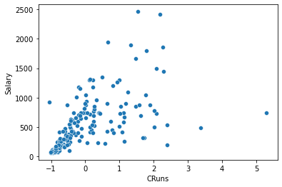
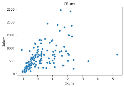
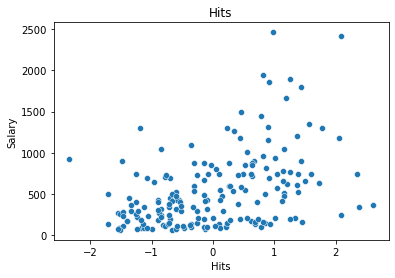
In this example, we only select two features: CRuns and Hits.

# choose features
x_spline = df_train[['CRuns', 'Hits']]

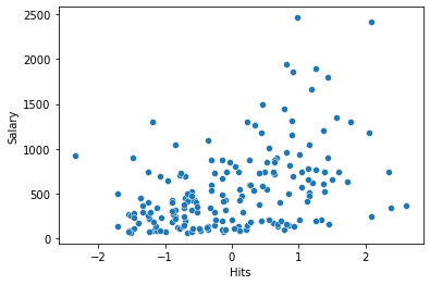
sns.scatterplot(x='CRuns', y='Salary', data=df_train);

sns.scatterplot(x='Hits', y='Salary', data=df_train);

Now we need to divide the range of X into K distinct regions (for every feature).
Within each region, a polynomial function is fit to the data.
In the statsmodels function BSplines, we need to provide df and degree:
- df: number of basis functions or degrees of freedom; should be equal in length to the number of columns of x; may be an integer if x has one column or is 1-D.
- degree: degree(s) of the spline; the same length and type rules apply as to df.

Degrees of freedom#

Instead of providing the number of knots, in statsmodels, we have to specify the degrees of freedom (df).
df defines how many parameters we have to estimate.
They have a specific relationship with the number of knots and the degree, which depends on the type of spline (see Stackoverflow):
In the case of B-splines:
- \(df=𝑘+degree\) if you specify the knots or
- \(𝑘=df−degree\) if you specify the degrees of freedom and the degree.

As an example:

A cubic spline (degree=3) with 4 knots (K=4) will have \(df=4+3=7\) degrees of freedom. If we use an intercept, we need to add an additional degree of freedom.
A cubic spline (degree=3) with 5 degrees of freedom (df=5) will have \(𝑘=5−3=2\) knots (assuming the spline has no intercept).

Note

The higher the degrees of freedom, the “wigglier” the spline gets because the number of knots is increased [James et al., 2021].

Model#

We want to fit a cubic spline (degree=3) with an intercept and three knots (K=3).
We use this values for both of our features (we also could use different values for one of the features).
This equals \(df=3+3+1=7\) for both of the features. This means that these degrees of freedom are used up by an intercept, plus six basis functions.

# create basis spline
bs = BSplines(x_spline, df=[7, 7], degree=[3, 3])

# fit model
reg = GLMGam.from_formula('Salary ~ CRuns + Hits', 
                                data=df_train, 
                                smoother=bs).fit()

# print results
print(reg.summary())

                 Generalized Linear Model Regression Results                  
==============================================================================
Dep. Variable:                 Salary   No. Observations:                  184
Model:                         GLMGam   Df Residuals:                   171.00
Model Family:                Gaussian   Df Model:                        12.00
Link Function:               identity   Scale:                          90949.
Method:                         PIRLS   Log-Likelihood:                -1304.8
Date:                Sat, 23 Apr 2022   Deviance:                   1.5552e+07
Time:                        14:34:52   Pearson chi2:                 1.56e+07
No. Iterations:                     3   Pseudo R-squ. (CS):             0.7307
Covariance Type:            nonrobust                                         
==============================================================================
                 coef    std err          z      P>|z|      [0.025      0.975]
------------------------------------------------------------------------------
Intercept    690.7415    160.681      4.299      0.000     375.813    1005.670
CRuns         98.7724     74.429      1.327      0.184     -47.106     244.651
Hits         -98.4006    112.343     -0.876      0.381    -318.588     121.787
CRuns_s0    -312.2840    407.009     -0.767      0.443   -1110.007     485.439
CRuns_s1    -206.0292    267.477     -0.770      0.441    -730.274     318.216
CRuns_s2     114.0089    284.464      0.401      0.689    -443.531     671.548
CRuns_s3     432.3174    322.183      1.342      0.180    -199.150    1063.785
CRuns_s4     208.7568    418.248      0.499      0.618    -610.994    1028.508
CRuns_s5    -216.1141    255.883     -0.845      0.398    -717.636     285.408
Hits_s0     -605.1108    497.421     -1.216      0.224   -1580.038     369.816
Hits_s1     -412.2057    280.829     -1.468      0.142    -962.620     138.208
Hits_s2     -244.4009    207.209     -1.179      0.238    -650.523     161.722
Hits_s3      109.4752    176.015      0.622      0.534    -235.508     454.458
Hits_s4      507.2235    255.672      1.984      0.047       6.116    1008.331
Hits_s5       68.8706    231.932      0.297      0.767    -385.708     523.450
==============================================================================

Plot#

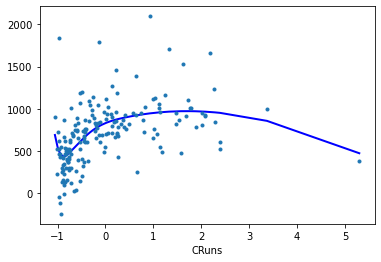
The results classes provide a plot_partial method that plots the partial linear prediction of a smooth component.
The partial residual or component plus residual can be added as scatter point with cpr=True.
Spline for feature CRuns:

reg.plot_partial(0, cpr=True, plot_se=False)

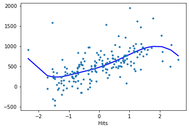
Spline for feature Hits:

reg.plot_partial(1, cpr=True, plot_se=False)

Model evaluation#

Training data#

# Training data
df_train['pred_train'] = reg.predict()
rmse_train = round(rmse(df_train['Salary'], df_train['pred_train']),4)

# plot training data
features = ['CRuns', 'Hits']

for i in features:
    g = sns.scatterplot(x=i, y='Salary', data=df_train)
    plt.title(i)
    plt.show();

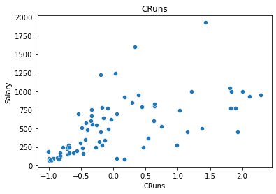
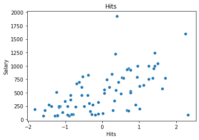
Test data#

We need to make sure that our test data falls inside the boundaries of the outermost knots (otherwise, we get an error)

# Obtain limits of training data features
x0_min = X_train['CRuns'].min()
x0_max = X_train['CRuns'].max()

x1_min = X_train['Hits'].min()
x1_max = X_train['Hits'].max()

# Only keep test data within training data limits
df_test = df_test[(df_test["CRuns"] > x0_min) & (df_test["CRuns"] < x0_max)]
df_test = df_test[(df_test["Hits"] > x1_min) & (df_test["Hits"] < x1_max)]

# plot test data
for i in features:
    g = sns.scatterplot(x=i, y='Salary', data=df_test)
    plt.title(i)
    plt.show();

# Obtain test RMSE
df_test['pred_test'] = reg.predict(df_test, exog_smooth= df_test[['CRuns', 'Hits']])
rmse_test = round(rmse(df_test['Salary'], df_test['pred_test']),4)

# Save model results
results = {"model": "GAM", "rmse_train": rmse_train, "rmse_test": rmse_test}

results

{'model': 'GAM', 'rmse_train': 290.7294, 'rmse_test': 272.6471}

Introduction to Regression Models

Generalized Additive Models (GAM)

Contents

Generalized Additive Models (GAM)#

Setup#

Data preparation#

Spline basis#

Degrees of freedom#

Model#

Plot#

Model evaluation#

Training data#

Test data#